Blog

A cloud migration service provider is a third-party engineering firm specializing in the architectural design and execution of moving a company's digital assets—applications, data, and infrastructure—from on-premises data centers or another cloud to a target cloud environment. An elite provider functions as a strategic technical partner, guiding you through complex architectural trade-offs, executing the migration with precision, and ensuring your team is equipped to operate the new environment effectively.

Defining Your Technical Blueprint Before You Search

Before initiating contact with any cloud migration provider, the foundational work must be internal. A successful migration is architected on a granular self-assessment, not a vendor's sales presentation. Engaging vendors without this internal technical blueprint is akin to requesting a construction bid without architectural plans or a land survey—it leads to ambiguous proposals, scope creep, and budget overruns.

This blueprint is your primary vetting instrument. It compels potential partners to respond to your specific technical and operational reality, forcing them beyond generic, templated proposals. The objective is to produce a detailed document that specifies not just your current state but your target state architecture and operational model.

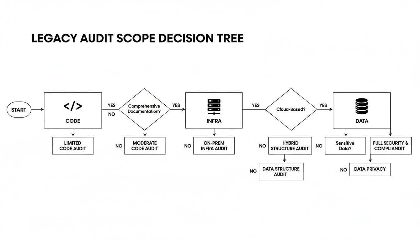
The diagram below outlines the sequential process for creating this technical blueprint.

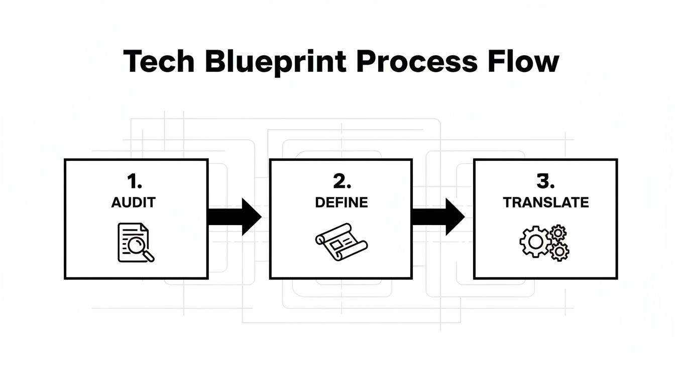
This sequence is non-negotiable: execute a comprehensive audit, define a precise target state, and then translate business objectives into quantifiable technical requirements.

Auditing Your Current Environment

Begin with a comprehensive technical audit of your existing infrastructure, applications, and network topology. This is not a simple inventory count; it's a deep-dive analysis of the interdependencies, performance characteristics, and security posture of your current systems.

Your audit must meticulously document:

• Application Portfolio Analysis: Catalog every application. Document its business criticality (Tier 1, 2, 3), architecture (monolithic, n-tier, microservices), and underlying technology stack (e.g., Java 8 with Spring Boot, Node.js 16, Python 3.9, .NET Framework 4.8). Specify database dependencies (e.g., Oracle 12c, PostgreSQL 11, MS SQL Server 2016).
• Dependency Mapping: Utilize automated discovery tools (e.g., AWS Application Discovery Service, Azure Migrate, or third-party tools like Device42) to map network communication paths and visualize dependencies between applications, databases, and external services. A failed migration often stems from an undiscovered dependency—a legacy authentication service or an overlooked batch job.
• Infrastructure Inventory: Document server specifications (CPU cores, RAM, OS version), storage types and performance (SAN IOPS, NAS throughput), network configurations (VLANs, firewall rules, load balancers), and current utilization metrics (CPU, memory, I/O, network bandwidth at P95 and P99). This data is critical for right-sizing cloud instances and avoiding performance bottlenecks or excessive costs.
• Security and Compliance Posture: Enumerate all current security tools (firewalls, WAFs, IDS/IPS), access control mechanisms (LDAP, Active Directory), and regulatory frameworks you are subject to (e.g., GDPR, HIPAA, PCI-DSS, SOX). These requirements must be designed into the target cloud architecture from the outset.

A thorough internal assessment is the prerequisite for understanding your current state and defining the success criteria for your migration.

Pre-Migration Internal Assessment Checklist

Assessment Area	Key Questions to Answer	Success Metric Example
Application Inventory	Which apps are mission-critical? Which can be retired? What are their API and database dependencies?	95% of Tier-1 applications successfully migrated with zero unplanned downtime during the cutover window.
Infrastructure & Performance	What are our current P95 CPU, memory, and storage IOPS utilization? Where are the performance bottlenecks under load?	Reduce average API endpoint response time from 450ms to sub-200ms post-migration.
Security & Compliance	What are our data residency requirements (e.g., GDPR)? What specific controls are needed for HIPAA or PCI-DSS?	Achieve a clean audit report against all required compliance frameworks within 90 days of migration.
Cost & TCO	What is our current total cost of ownership (TCO), including hardware refresh cycles, power, and personnel?	Reduce infrastructure TCO by 15% within the first 12 months, verified by cost allocation reports.
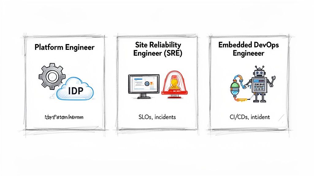
Skills & Team Readiness	Does our team possess hands-on expertise with IaC (Terraform), container orchestration (Kubernetes), and cloud-native monitoring?	Internal team can independently manage 80% of routine operational tasks (e.g., deployments, scaling events) within 6 months.

This checklist serves as a starting point for constructing the detailed blueprint a potential partner must analyze to provide an intelligent proposal.

Translating Business Goals into Technical Objectives

With a complete audit, you can translate high-level business goals into specific, measurable, achievable, relevant, and time-bound (SMART) technical objectives. A goal like "reduce costs" is unactionable for an engineering team.

Here is a practical breakdown:

• Business Goal: Improve application performance and user experience.
  • Technical Objective: Achieve a P95 response time of sub-200ms for key API endpoints (/api/v1/users, /api/v1/orders). This will be accomplished by refactoring the monolithic application into discrete microservices deployed on a managed Kubernetes cluster (e.g., EKS, GKE, AKS) with auto-scaling enabled.
• Business Goal: Increase development agility and deployment frequency from monthly to weekly.
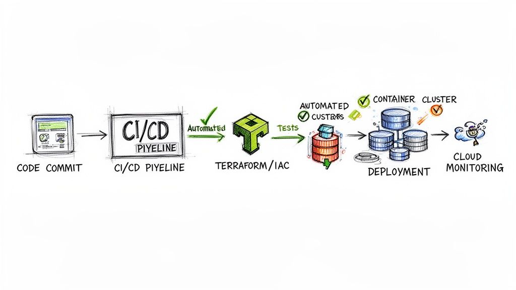
  • Technical Objective: Implement a complete CI/CD pipeline using Jenkins or GitLab CI, leveraging Terraform for Infrastructure as Code (IaC) to enable automated, idempotent deployments to staging and production environments upon successful merge to the main branch.
• Business Goal: Cut infrastructure operational overhead by 30%.
  • Technical Objective: Adopt a serverless-first architecture for all new event-driven services using AWS Lambda or Azure Functions, eliminating server provisioning and management for these workloads.

This translation process converts business strategy into an executable engineering plan. Presenting these specific objectives ensures a substantive, technical dialogue with a potential cloud migration service provider.

For assistance in defining these targets, a dedicated cloud migration consultation can refine your strategy before you engage a full-service provider. It is also crucial to fully comprehend what cloud migration entails for your specific business context to set realistic expectations.

Crafting an RFP That Exposes True Expertise

A generic Request for Proposal (RFP) elicits generic, boilerplate responses. To identify a true technical partner, your RFP must act as a rigorous technical filter—one that forces a cloud migration service provider to demonstrate its engineering depth, not its marketing prowess.

Think of it as providing a detailed schematic and asking how a contractor would execute the build, rather than just asking if they can build a house. A well-architected RFP is your most critical vetting instrument.

Articulating Your Technical Landscape

Your RFP must provide a precise, unambiguous snapshot of your current state and target architecture. Ambiguity invites assumptions, which are precursors to scope creep and budget overruns.

Be specific about your current technology stack. Do not just state "databases"; specify "a sharded MySQL 5.7 cluster on bare metal, managing approximately 2TB of transactional data with a peak load of 5,000 transactions per second." This level of detail is mandatory.

Clearly define your target architecture by connecting business goals to specific cloud services and methodologies:

• For containerization: "Our target state is a microservices architecture. Propose a detailed plan to containerize our primary monolithic Java application and deploy it on Google Kubernetes Engine (GKE). Your proposal must detail your approach to ingress (e.g., GKE Ingress, Istio Gateway), service mesh implementation (e.g., Istio, Linkerd), and secrets management (e.g., Google Secret Manager, HashiCorp Vault)."
• For serverless functions: "We are refactoring our nightly batch processing jobs into event-driven serverless functions. Describe your experience with Azure Functions using the Premium plan. Detail how you would handle triggers from Azure Blob Storage, implement idempotent logic, manage error handling via dead-letter queues, and ensure secure integration with our on-premises data warehouse."
• For compliance: "Our application processes Protected Health Information (PHI). The proposed architecture must be fully HIPAA compliant. Explain your precise configuration for logging (e.g., AWS CloudTrail, Azure Monitor), encryption at rest and in transit (e.g., KMS, TLS 1.2+), and IAM policies to meet these standards."

This specificity forces providers to engage in architectural problem-solving, not just marketing.

Demanding Specifics on Methodology and Governance

An expert partner brings a proven, battle-tested methodology. Your RFP must probe this area aggressively to distinguish strategic executors from mere order-takers. You are shifting the evaluation from what they will build to how they will build, test, and deploy it.

A provider's response to questions about methodology is often the clearest indicator of their experience. Vague answers suggest a lack of a battle-tested process, while detailed, opinionated responses show they've navigated complex projects before.

Challenge them to define their process for core migration tasks. You need evidence of a structured, repeatable methodology for secure and efficient execution. As managing these relationships is a discipline, familiarize your team with vendor management best practices.

Structuring Questions for Clarity

Frame questions to elicit concrete, comparable, and technical answers. Avoid open-ended prompts that invite marketing fluff.

IaC and Automation Proficiency:
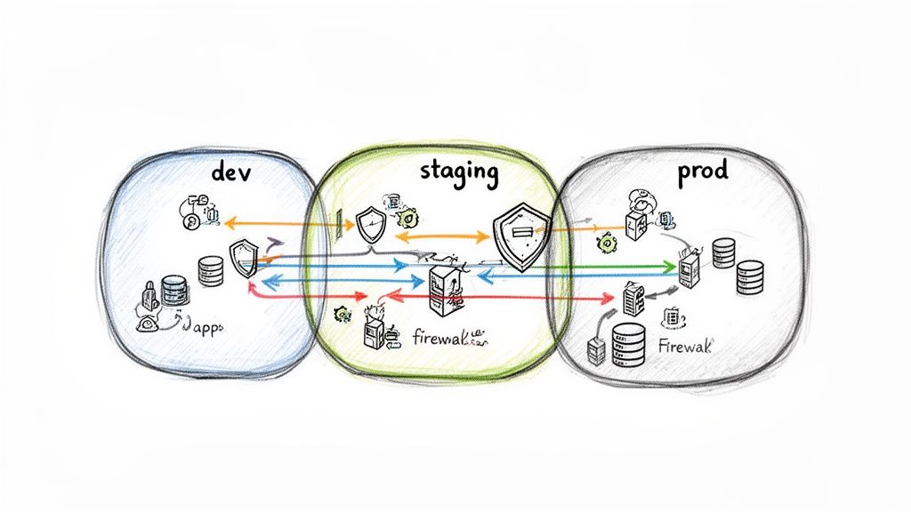
"Describe your team's proficiency with Terraform. Provide a code sample illustrating how you would structure Terraform modules to manage a multi-environment (dev, staging, prod) setup in AWS. The sample should demonstrate how you enforce consistent VPC, subnet, and security group configurations and manage state."

Migration Strategy Justification:
"For our legacy CRM application (a .NET 4.5 monolith with a SQL Server backend), would you recommend a Rehost ('lift-and-shift') or a Refactor approach? Justify your choice with a quantitative analysis weighing initial downtime and cost against long-term TCO and operational agility. What are the primary technical risks of your chosen strategy and your mitigation plan?"

Project Governance and Communication:
"Detail your proposed project governance model. Specify the cadence for technical review meetings. How will you track progress against milestones using quantitative metrics (e.g., velocity, burndown charts)? What specific tools (e.g., Jira, Azure DevOps, Confluence) will be used for ticket management, documentation, and communication with our engineering team?"

By demanding this level of technical detail, your RFP becomes a powerful diagnostic tool, quickly separating providers with genuine, hands-on expertise from those with only proposal-writing skills.

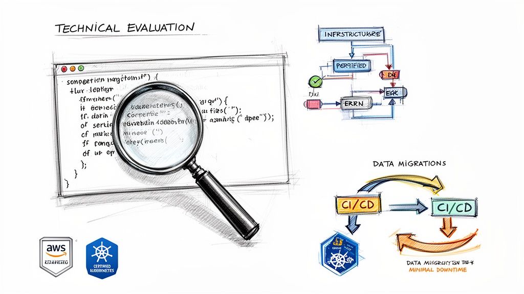
Evaluating a Provider's Technical Chops and Strategy

With proposals in hand, the next phase is a rigorous technical evaluation to distinguish true engineering experts from proficient sales teams. A compelling presentation is irrelevant if the provider lacks the technical depth to execute your project's specific requirements.

The objective is not to select the provider with the most certifications but to find a team whose demonstrated, hands-on experience aligns with your technology stack, scale, and architectural goals.

Beyond the Case Study Glossy

Every provider will present curated case studies. Your task is to dissect them for technical evidence, not just business outcomes. If your project involves containerizing a Java monolith on Azure Kubernetes Service (AKS), a case study about a simple "lift-and-shift" of VMs to AWS is not relevant evidence of capability.

Scrutinize their past projects with technical granularity:

• Scale and Complexity: Did they migrate a 10TB multi-tenant OLTP database or a 100GB departmental database? Was it a single, stateless application or a complex system of 50+ interdependent microservices with convoluted data flows?
• Tech Stack Parallels: Demand evidence of direct experience with your core technologies. If you run a high-throughput PostgreSQL cluster, a provider whose expertise is limited to MySQL or Oracle will be learning on your project.
• Problem-Solving Details: The most valuable case studies are post-mortems, not just success stories. They should detail the technical obstacles encountered and overcome. How did they resolve an unexpected network latency issue post-migration? How did they script a complex data synchronization process for the final cutover?

These details reveal whether their experience is truly applicable or merely adjacent.

Verifying Team Expertise and Certifications

A provider is the sum of the engineers assigned to your project. Request the profiles and certifications of the specific team members who will execute the work. Certifications serve as a validated baseline of knowledge.

Key credentials to look for include:

• Cloud Platform Specific: AWS Certified Solutions Architect – Professional or Microsoft Certified: Azure Solutions Architect Expert demonstrates deep platform-specific architectural knowledge.
• Specialized Skills: For container orchestration, a Certified Kubernetes Administrator (CKA) or Certified Kubernetes Application Developer (CKAD) is essential.
• Infrastructure as Code (IaC): The HashiCorp Certified: Terraform Associate certification validates foundational automation skills.

Certifications prove foundational knowledge, but they don't replace hands-on experience. During technical interviews, ask engineers to describe a complex problem they solved using the skills validated by their certification. Their answer will reveal their true depth of expertise.

Probe their practical, in-the-weeds experience. Ask them to whiteboard a CI/CD pipeline architecture using GitLab CI for a containerized application. Ask about their preferred methods for managing secrets in Kubernetes (e.g., Sealed Secrets, External Secrets Operator, Vault). The fluency and technical depth of their answers are your best indicators of real expertise.

The market is accelerating, with companies achieving operational efficiency gains of up to 30% and reducing IT infrastructure costs by up to 50%. The hybrid cloud market is growing at an 18.7% CAGR as organizations optimize workload placement for performance, cost, and compliance. The official AWS blog details why a migration inflection point is approaching.

Analyzing the Proposed Migration Methodology

Dissect their proposed migration strategy. A premier provider will justify their approach with a clear, data-driven rationale linked directly to your stated technical and business objectives. They must present a detailed plan for data migration with minimal downtime and a comprehensive strategy for testing and validation.

Ask pointed, technical questions that test their problem-solving capabilities:

1. Data Migration: "Present your specific technical plan for migrating our primary 2TB PostgreSQL database with a maximum downtime window of 15 minutes. Detail the tools (e.g., AWS DMS, native replication), the sequence of events, and the rollback procedure if validation fails post-cutover."
2. Testing and Validation: "Describe your testing strategy. How will you automate integration, performance (load testing), and security (penetration testing) in the new cloud environment before the final cutover? What specific metrics and SLOs will define a successful test?"
3. Contingency Planning: "Walk me through a failure scenario. Assume that mid-migration, we discover a critical, undocumented hard-coded IP address in a legacy application. What is your process for diagnosing, adapting the plan, and communicating the impact on the timeline and budget?"

Their responses to these questions will provide the clearest insight into their real-world competence. A confident, detailed response indicates experience; vague answers are a significant red flag.

Comparing the 6 R's of Migration Strategy

A provider's plan will be based on the "6 R's" of cloud migration. Understanding these allows you to critically evaluate their proposal and challenge their choices for each application.

Strategy	Description	Best For	Key Consideration
Rehost	"Lift-and-shift." Moving applications as-is by migrating VMs or servers.	Rapid, large-scale migrations where redesign is not immediately feasible.	Fails to leverage cloud-native features; can result in higher long-term TCO.
Replatform	"Lift-and-reshape." Making minor cloud optimizations without changing the core architecture.	Gaining immediate cloud benefits (e.g., moving from self-managed MySQL to Amazon RDS) without a full rewrite.	An intermediate step that can add complexity if not part of a longer-term refactoring plan.
Repurchase	Moving to a SaaS solution.	Replacing on-premises commodity software (e.g., CRM, HR systems) with a cloud-native alternative.	Requires data migration, user retraining, and potential business process re-engineering.
Refactor	Re-architecting an application to be cloud-native, often using microservices and serverless.	Maximizing cloud benefits: scalability, resilience, performance, and cost-efficiency.	Highest upfront cost and effort; requires significant software engineering resources.
Retire	Decommissioning applications that are no longer needed.	Reducing complexity, cost, and security surface area by eliminating obsolete systems.	Requires thorough dependency analysis to ensure no critical business functions are broken.
Retain	Keeping specific applications on-premises.	Hybrid cloud strategies, applications with extreme low-latency requirements, or those that cannot be moved.	Necessitates a robust strategy for hybrid connectivity and integration (e.g., VPN, Direct Connect).

An expert partner will propose a blended strategy, applying the appropriate "R" to each application based on its business value, technical architecture, and your overall goals. They must be able to defend each decision with data.

Getting Serious About Security, Compliance, and SLAs

A migration is a failure if it introduces security vulnerabilities or violates compliance mandates, regardless of application uptime. A rigorous evaluation of a provider's security practices and service level agreements (SLAs) is non-negotiable. This involves understanding their methodology for engineering secure cloud environments from the ground up.

Kicking the Tires on Core Security Practices

A provider's security expertise is demonstrated through technical details. Drill down on their approach to Identity and Access Management (IAM). They must articulate how they implement the principle of least privilege. Ask for examples of IAM roles and policies they would construct for developers, applications (via service accounts), and CI/CD pipelines, ensuring each has the minimum required permissions.

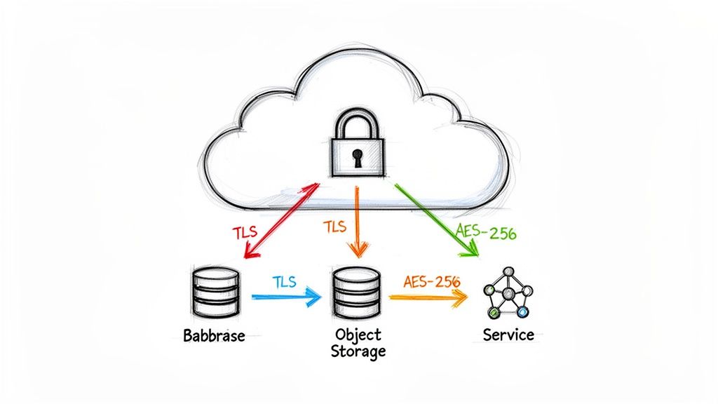
Data encryption is paramount. They should detail their standards for encryption in transit (e.g., enforcing TLS 1.2 or higher) and at rest (e.g., using AWS KMS with customer-managed keys or Azure Key Vault). Ask about their process for key rotation and lifecycle management.

Probe their network architecture design. Discuss their methodology for designing secure Virtual Private Clouds (VPCs) or Virtual Networks (VNets), including their strategies for multi-tier subnetting (public, private, database), configuration of network access control lists (NACLs), and the principle of default-deny for security groups.

Your partner must be an expert in mastering cloud infra security—it is the foundation of a modern, resilient business.

Navigating the Maze of Regulatory Compliance

If your business operates under specific regulatory frameworks, the provider's direct experience is critical. A generic claim of "compliance experience" is insufficient. You need evidence they have successfully implemented and audited environments under your specific mandate.

• Healthcare (HIPAA): Request a detailed architectural diagram of a HIPAA-compliant environment they have built. They should be able to discuss implementing Business Associate Agreements (BAAs) with the cloud vendor and configuring services like AWS CloudTrail or Azure Monitor for immutable logging of access to Protected Health Information (PHI).
• Finance (PCI DSS): Scrutinize their experience with segmenting Cardholder Data Environments (CDE). They must explain precisely how they use network segmentation, firewall rules, and intrusion detection systems to isolate the CDE and meet stringent PCI requirements.
• Data Privacy (GDPR/CCPA): Discuss their implementation of data residency controls and their technical strategies for fulfilling "right to be forgotten" requests within a distributed cloud architecture.

The demand for cloud migration services is driven by these complex security and compliance requirements. North America leads the market because organizations are leveraging advanced cloud security features to adhere to frameworks like HIPAA, GDPR, and CCPA.

If a provider cannot fluently discuss the technical controls specific to your compliance framework, they are not qualified. This area demands proven, hands-on expertise.

Decoding the Service Level Agreement (SLA)

Look beyond the headline 99.99% uptime promise in the Service Level Agreement (SLA). The fine print defines the true nature of the commitment. A robust SLA is your primary tool for accountability.

Our cloud security checklist provides a comprehensive guide, but your SLA review must cover these technical specifics:

• Support Response Times: What are the guaranteed response and resolution times for different severity levels (e.g., Sev1, Sev2, Sev3)? A "24-hour response" for a critical production outage (Sev1) is unacceptable.
• Remediation Processes: The agreement must define Mean Time to Resolution (MTTR) targets. What are the provider's contractual obligations for resolving an issue once acknowledged?
• Financial Penalties: What are the specific service credits or financial penalties for failing to meet the SLA? The penalties must be significant enough to incentivize performance.

The signed contract is the final step in your vetting process. It must codify a partnership that protects your digital assets and contractually binds the provider to their commitments.

Planning for Life After Migration

The migration cutover is not the finish line; it is the starting point for cloud operations. Many organizations execute a successful migration only to face runaway costs and operational instability. A premier cloud migration service provider anticipates this and ensures a structured transition to your team.

The post-migration phase is where the true value of the partnership is realized. The objective is not merely to migrate you to the cloud but to empower your team to operate and optimize the new environment effectively.

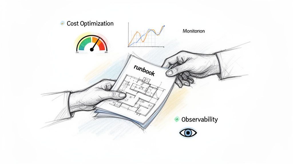
Structuring a Successful Technical Handover

A proper handover is a formal knowledge transfer process, not a simple email. Your provider must deliver a comprehensive package of documentation, code, and training.

Insist on these deliverables:

• Architectural Diagrams: Detailed, up-to-date diagrams of the cloud architecture, including VPC/VNet layouts, subnets, security groups, service integrations, and data flow diagrams.
• Runbooks: Step-by-step operational procedures for common tasks and incident response. Examples include: "How to perform a database point-in-time restore," "Procedure for responding to a high CPU alert on the Kubernetes cluster," and "Disaster recovery failover process."
• IaC Repository: Full access to the well-documented Terraform or CloudFormation repository used to provision the infrastructure. The code should be modular, commented, and follow best practices.

Documentation alone is insufficient. Demand hands-on training sessions where your engineers work alongside the provider's team to learn the new operational workflows, CI/CD processes, and monitoring tools.

Defining Your Ongoing Partnership Model

Complete disengagement is often impractical. Transition to a long-term relationship model that provides strategic value without creating operational dependency.

Common models include:

• Managed Services: The provider assumes responsibility for day-to-day operations, including monitoring, patching, and incident response. Ideal for teams that need to focus on application development.
• Advisory Retainer: You retain access to their senior architects for a fixed number of hours per month for strategic guidance on cost optimization, security posture, or adopting new cloud services.
• Project-Based Engagements: You re-engage the provider for specific, well-defined projects, such as implementing a new disaster recovery strategy or building out a data analytics platform.

The optimal model depends on your in-house skill set and long-term strategic goals.

The most successful post-migration strategies I've witnessed involve a gradual transfer of ownership. The provider starts by managing everything, then moves to a co-pilot role, and finally transitions to an on-demand advisor as your team's confidence and expertise grow.

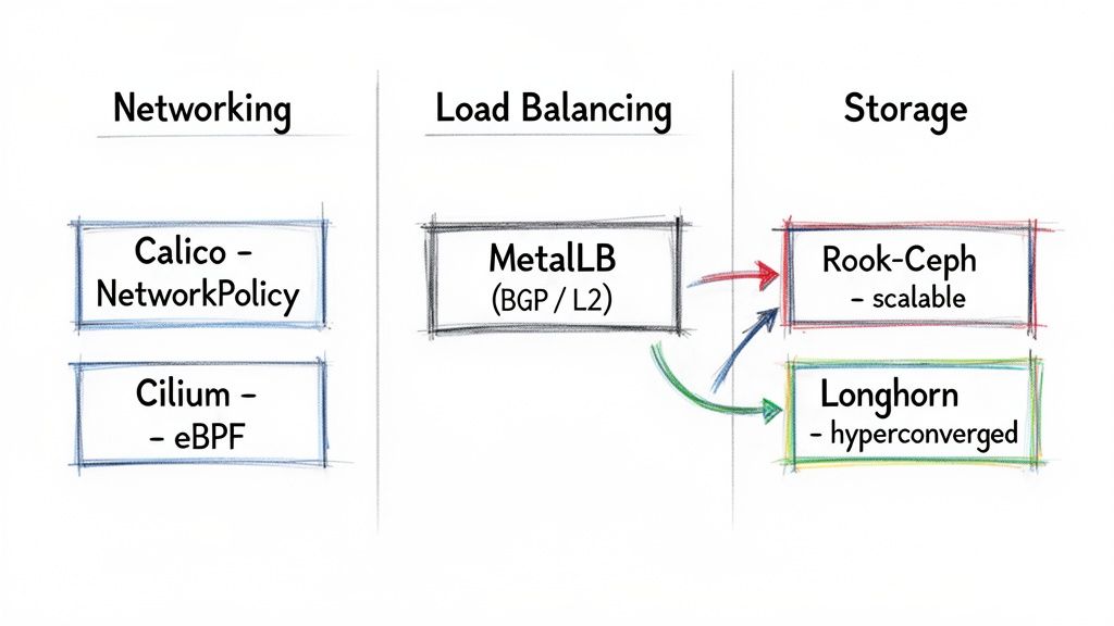
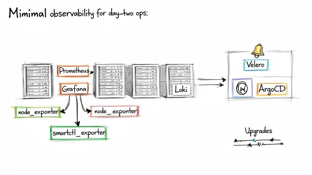
Implementing FinOps and Observability

Two disciplines are critical for long-term cloud success: FinOps (Financial Operations) and observability. Your provider should help establish a strong foundation for both before the handover.

For FinOps, this involves implementing tools and processes for cloud financial management. This includes resource tagging strategies to attribute costs to specific teams or projects, setting up automated policies to decommission idle resources (e.g., using AWS Lambda or Azure Automation), and creating dashboards to track spend against budget. They should also provide an analysis for purchasing Reserved Instances or Savings Plans.

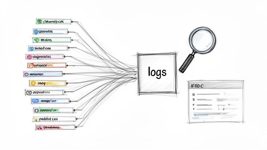
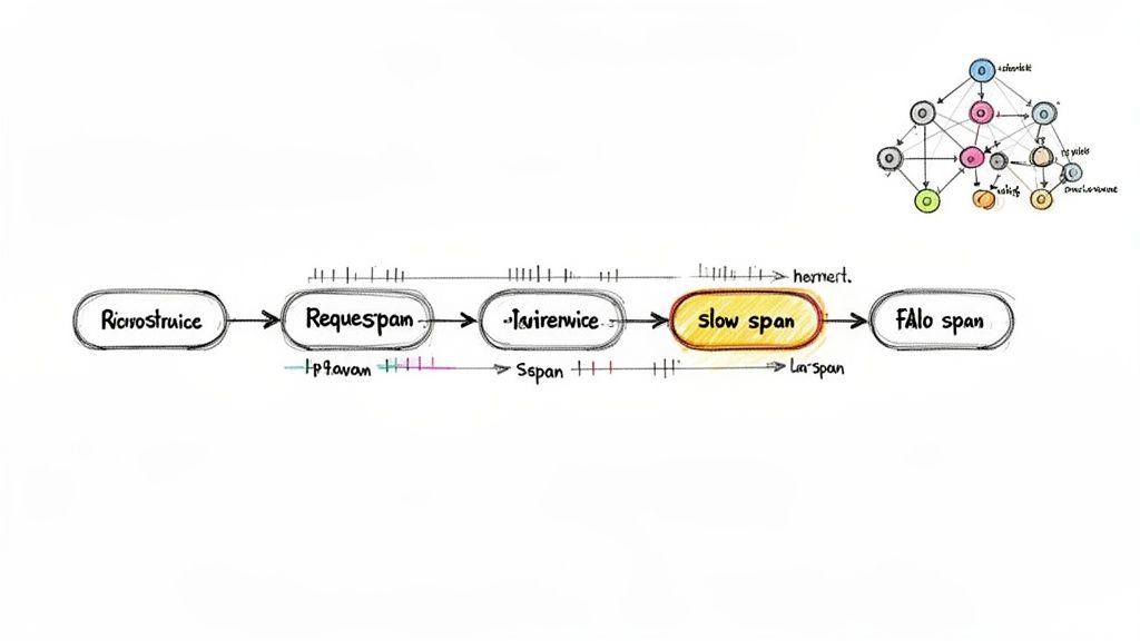
For observability, this means moving beyond basic metrics (CPU, memory) to a comprehensive understanding of system health through metrics, logs, and traces. This often involves instrumenting applications and infrastructure with tools like Prometheus for metrics, Loki or the ELK Stack for logs, and Jaeger or OpenTelemetry for tracing. A good partner will help you configure dashboards and alerts based on Service Level Objectives (SLOs) that reflect the end-user experience.

Frequently Asked Questions

Embarking on a cloud migration project brings many technical and strategic questions. Here are answers to some of the most common inquiries.

What Common Mistakes Should I Avoid When Choosing a Provider?

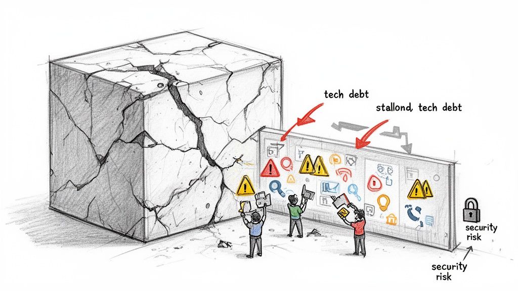
The most common and costly mistake is selecting a provider based solely on the lowest price. This often leads to technical debt, security vulnerabilities, and expensive rework when the initial migration fails to meet performance or operational requirements.

Another critical error is failing to perform deep technical diligence on a provider's case studies and references. You must verify that they have successfully executed projects of similar technical complexity, scale, and compliance requirements.

Other technical red flags include:

• A "one-size-fits-all" plan: A competent provider will insist on a paid discovery phase to conduct a thorough audit before proposing a solution. A generic template is a sign of inexperience.
• A vague Statement of Work (SOW): The SOW must precisely define the scope, technical deliverables, success criteria (SLOs/SLAs), and operational handover plan. Ambiguity leads to scope creep and disputes.
• Neglecting post-migration operations: A project plan that ends at cutover is incomplete. Failing to plan for knowledge transfer, FinOps implementation, and ongoing operational support sets your internal team up for failure.

How Long Does a Typical Cloud Migration Project Take?

There is no "typical" timeline without a detailed assessment. The duration varies significantly based on complexity and the chosen migration strategy.

A simple Rehost ("lift-and-shift") of a few dozen VMs might be completed in several weeks. However, a complex Refactor of a core monolithic application into cloud-native microservices on Kubernetes can take 6 to 18 months or more.

An experienced cloud migration provider will never provide a definitive timeline upfront. They will propose a phased approach with clear milestones and deliverables for each stage: Assessment, Planning, Execution, and Optimization.

Factors that heavily influence the timeline include the volume of data to be migrated, the complexity of application dependencies, the level of test automation required, and the extent to which Infrastructure as Code is adopted.

Is a Cloud Migration Specialist Different from an MSP?

Yes, their core competencies and engagement models are distinct, though some firms offer both services.

A cloud migration service provider is a project-based specialist. Their expertise is focused on the one-time event of planning and executing the migration from a source to a target environment. The engagement is finite, concluding with the successful handover of the new cloud infrastructure to your team.

A Managed Service Provider (MSP) focuses on long-term, ongoing operations. They engage after the migration is complete to manage the day-to-day operational tasks of the cloud environment, which typically include:

• 24/7 monitoring and incident response (NOC/SOC functions)
• Security posture management and compliance auditing
• OS and application patching
• Cost monitoring and optimization

It is critical to evaluate a provider's expertise in each domain separately. The skills required for complex architectural design and migration are different from those required for efficient daily cloud operations.

How Do I Create an Accurate Budget for a Cloud Migration?

A comprehensive budget extends beyond the provider's professional services fees. It must account for several key cost categories.

First, the provider's fees, structured as either a fixed-price contract for a well-defined scope or a time-and-materials (T&M) model for more exploratory refactoring projects.

Second, the cloud consumption costs during and after migration. Your provider should help you create a detailed forecast using tools like the AWS Pricing Calculator or Azure TCO Calculator. This forecast must include compute, storage, networking, data egress fees, and any managed services (e.g., RDS, EKS).

Third, account for third-party software and tooling licenses. This may include migration tools, new security platforms (e.g., WAF, CWPP), or observability platforms (e.g., Datadog, New Relic).

Finally, budget for the internal cost of your own team's time. Your engineers and project managers will be heavily involved in the process. Investing in a paid discovery or assessment phase is the most reliable method for gathering the data needed to build an accurate, comprehensive budget.

---

At OpsMoon, we bridge the gap between strategy and execution. Our Experts Matcher connects you with the top 0.7% of global DevOps talent to ensure your cloud migration is not just completed, but masterfully executed with a clear plan for post-migration success. Plan your project with a free work planning session to build a clear roadmap for your cloud journey. https://opsmoon.com

CI/CD consulting isn't just about tool installation. It’s the expert-led engineering service that re-architects and implements your automated software delivery pipelines. The objective is to replace slow, error-prone manual processes with a high-velocity, resilient system—a critical move for any organization that needs to innovate faster and slash operational risk by shipping reliable code.

What Is CI/CD Consulting?

Many engineering teams fall into the trap of viewing CI/CD as a tooling problem. The reality is that a robust CI/CD pipeline is the central nervous system for modern software delivery. It dictates the velocity, quality gates, and security posture for every single deployment.

An old-school software process resembles an artisan workshop: skilled developers hand-crafting each component. It produces software, but it's slow, wildly inconsistent, and dangerously prone to human error. Each deployment is a high-stakes event, managed with manual checklists and hope-driven engineering.

CI/CD consulting provides the architectural and software engineering expertise to replace that workshop with a fully automated, observable, and resilient software factory. A consultant acts as the lead systems architect, blue-printing every stage of the software development lifecycle (SDLC) to eliminate toil and reduce cognitive load.

Re-Architecting Your Development and Deployment Process

The goal extends far beyond simple automation. We’re talking about a fundamental re-architecture of the workflow, from the moment a developer runs git commit to the second that code is handling live production traffic.

This transformation focuses on engineering a system that is:

• Fast: Automating builds, static analysis, unit/integration testing, and deployments to shrink the cycle time from a pull request to a production release. This means reducing the time it takes to get feedback on a change from hours or days to minutes.
• Reliable: Implementing immutable infrastructure and version-controlled, repeatable deployment processes to eliminate the "it works on my machine" class of errors and drastically cut down on deployment failures.
• Secure: Embedding automated security controls directly into the pipeline (DevSecOps) to detect vulnerabilities, secrets, and dependency issues early, not during a post-breach incident response.

This is why high-performing organizations no longer view CI/CD as an IT cost center. They recognize it as a fundamental investment in their ability to out-maneuver competitors and respond to market demands in near real-time.

A well-designed CI/CD pipeline isn't just about shipping code faster. It's about building an engineering culture of quality, feedback, and continuous improvement, where developers can focus on innovation instead of manual, repetitive tasks.

The demand for this level of expertise is accelerating. Between 2023 and 2034, global spending on CI/CD tools and services is projected to grow at a compound annual rate of 15–19%. This is no longer a niche practice; it's a mainstream strategic investment for any company building software. You can discover more insights about this growing market and its massive projected expansion.

Diagnosing a Broken Software Delivery Lifecycle

Before you can architect a solution, you must diagnose the specific failures in the system. A broken software delivery lifecycle (SDLC) is rarely a single catastrophic event. It’s a slow accumulation of technical debt, process flaws, and brittle infrastructure that grinds engineering velocity to a halt.

The symptoms manifest as daily, high-friction frustrations for your engineering teams, not just "slow releases."

These issues are more than minor annoyances. They directly inhibit innovation, crater developer morale, and kill product velocity. Pinpointing these specific failure modes is the first step in understanding the value that expert ci cd consulting can deliver.

The Anatomy of 'Merge Hell'

A classic symptom of a broken CI process is "merge hell." This state occurs when feature branches diverge significantly from the main branch over long periods, making the eventual integration a high-risk, bug-prone exercise.

Your most senior engineers, who should be architecting new systems, are instead forced to spend hours—sometimes days—resolving complex merge conflicts and untangling dependencies. This is a massive productivity sink that burns out top talent and stalls forward momentum. A core goal of CI is to integrate frequently (git pull --rebase becomes a reflex) to prevent this divergence.

Configuration Drift and Deployment Anxiety

Another clear indicator is the friction caused by environmental inconsistency. When development, staging, and production environments are configured manually, they inevitably experience configuration drift. This is the root cause of the infamous "it works on my machine" problem, which erodes trust between development, QA, and operations.

This inconsistency breeds a culture of deployment anxiety. Each release becomes a high-stakes, "all hands on deck" event managed by manual runbooks and last-minute heroics. The process is so painful and risky that teams actively avoid deploying, directly contradicting the principles of agility.

A healthy CI/CD pipeline transforms deployments from a source of fear into a routine, low-risk, and fully automated business-as-usual activity. It makes releasing new value to customers a non-event.

Manual Security Gates and Undetected Vulnerabilities

In a broken SDLC, security is often treated as a final, manual gate before production. This approach is not just slow; it's dangerously ineffective. Manual code reviews are prone to human error and cannot scale with the pace of modern development.

The result is that vulnerabilities are deployed to production. Common but critical issues, like hardcoded secrets in source code (AWS_SECRET_ACCESS_KEY="..."), go completely undetected. Research consistently shows that internal repositories can contain 8-10 times more secrets than public ones, creating a massive, unmonitored attack surface.

A proper DevSecOps pipeline integrates automated security scanning at multiple stages. It catches these issues early, providing developers with immediate feedback long before the code is merged.

If these symptoms are painfully familiar, you're not alone. Each represents a clear opportunity for improvement through intelligent automation and process re-engineering—the exact focus of a CI/CD consulting engagement.

What You Actually Get: Core CI/CD Consulting Deliverables

When you hire a CI/CD consultant, you're not just buying meetings and slide decks. You're investing in tangible engineering assets that enable your business to ship software faster and more reliably. The engagement moves beyond theory and into producing concrete, technical deliverables that solve real-world problems in your SDLC.

This is a structured process for engineering a better delivery engine, starting with a deep diagnosis and ending with a fully automated pipeline your team can own, operate, and extend with confidence.

A Data-Driven Assessment and Actionable Technical Roadmap

The first deliverable is a comprehensive DevOps maturity assessment. You cannot build the right solution without a precise understanding of the current state. This involves a deep technical audit of existing tools, workflows, code repositories, branching strategies, infrastructure, and deployment artifacts.

From this audit, the consultant produces a phased implementation roadmap. This is a strategic, step-by-step plan that prioritizes actions based on impact versus effort. It clearly defines technical milestones (e.g., "Phase 1: Implement Pipeline as Code for Service X"), success metrics (e.g., "Reduce build time from 45 mins to <10 mins"), and ensures every engineering action aligns with strategic business goals.

The roadmap is the architectural blueprint for your entire CI/CD transformation. It’s all about delivering incremental value at each stage, preventing a risky "big bang" approach that stalls progress and leaves everyone waiting for results.

So, how do high-level business pains map to the actual work a consultant does? Here’s a technical breakdown:

Mapping Business Problems To CI/CD Consulting Deliverables

This table shows how common frustrations in software delivery are directly addressed by specific, technical solutions from a CI/CD expert.

Business Problem	Technical Root Cause	CI/CD Consulting Deliverable
"Our releases are slow and unpredictable."	Manual deployment processes, inconsistent environments, lack of automation.	Automated Deployment Pipelines defined with Pipeline as Code (Jenkinsfile, gitlab-ci.yml, GitHub Actions YAML).
"Bugs keep slipping into production."	Insufficient testing, no automated quality gates, long feedback loops for devs.	Integrated Quality Gates (unit tests, static code analysis with SonarQube, code coverage reports) and a Test Automation Framework.
"Our developers are bogged down by process."	Manual environment setup, complex build configurations, siloed security reviews.	Ephemeral Test Environments (spun up per PR via Terraform/Pulumi) and a Self-Service Developer Platform.
"We had a security breach from a leaked key."	Secrets are hardcoded in source control, no automated scanning.	DevSecOps Implementation with automated secrets scanning (e.g., Git-leaks) and SAST (e.g., Snyk, Checkmarx).
"Our teams can't easily reproduce issues."	"Works on my machine" syndrome, configuration drift between environments.	Version-Controlled Environments using Infrastructure as Code (IaC) tools like Terraform.

As you can see, the deliverables are direct, technical solutions to frustrating and costly business problems. Let's dig into what some of those key deliverables look like.

Version-Controlled Pipeline as Code Artifacts

A core principle of modern DevOps is treating your pipeline configuration as code. A key deliverable from any credible consultant is Pipeline as Code (PaC).

This means your entire build, test, and deployment logic is defined in version-controlled text files that live alongside your application code in Git. This provides:

• Traceability: Every change to the pipeline is a Git commit. You can see who changed what, when, and why.
• Repeatability: Onboard a new microservice by reusing a standardized pipeline template. This eliminates configuration drift between services.
• Disaster Recovery: If your CI server is lost, you can rebuild the entire pipeline configuration from code in minutes.

Your consultant will deliver these artifacts using the standard formats for your CI/CD platform, like .gitlab-ci.yml files for GitLab CI/CD, workflow YAMLs for GitHub Actions, or Jenkinsfiles (declarative or scripted) for Jenkins.

Built-in Security and Quality Gates

In a modern SDLC, security is not a final step; it's a continuous process. A critical set of deliverables involves embedding automated security and quality checks directly into the pipeline itself.

This is the core of DevSecOps. The consultant will implement tools to catch vulnerabilities before code is merged. Key deliverables include:

• Static Application Security Testing (SAST): Tools like SonarQube or Snyk Code scan source code for known anti-patterns and vulnerabilities.
• Dynamic Application Security Testing (DAST): Tools like OWASP ZAP probe the running application in a test environment to find exploitable vulnerabilities.
• Secrets Scanning: Automated checks (e.g., truffleHog, gitleaks) that run pre-commit or on the CI server to prevent developers from committing credentials.

Beyond security, they will implement automated quality gates—such as enforcing unit test coverage thresholds and running linters—to ensure every commit meets your team’s engineering standards. There are many ways to approach CI/CD pipeline optimization to ensure these gates are fast and effective.

Automated Test Environments and Artifact Management

Finally, a consultant builds the supporting infrastructure for a truly automated workflow. This includes setting up ephemeral testing environments—fully functional, on-demand environments created automatically for every pull request. This allows developers and QA to test changes in a clean, isolated, production-like setting, which is one of the most powerful CI/CD pipeline best practices.

Another crucial component is configuring an artifact repository using tools like JFrog Artifactory or Sonatype Nexus. This provides a centralized, versioned storage for all build outputs (Docker images, Java JARs, npm packages), ensuring you have a single source of truth for every deployable component.

How to Measure the ROI of Your CI/CD Investment

A world-class CI/CD pipeline is a significant engineering asset. To justify the investment, you must speak the language of the business: Return on Investment (ROI).

Proving the value of CI/CD isn't about vague promises like "we'll go faster." It's about drawing a direct line from specific technical improvements to measurable business outcomes.

To achieve this, we rely on the four key DORA metrics. These are not vanity metrics for engineers; they are the industry standard for measuring the performance of elite software delivery teams. A successful CI/CD consulting engagement will demonstrably improve every single one.

From Technical Metrics to Financial Gains

Each DORA metric provides critical data about your team's velocity and stability. By establishing a baseline before a CI/CD implementation and tracking these metrics afterward, you can build a powerful, data-backed business case.

• Deployment Frequency: How often do you successfully release to production? Elite teams deploy on-demand, multiple times a day.
• Lead Time for Changes: What is the median time from code commit to production release? This is a raw measure of your entire delivery process efficiency.
• Change Failure Rate: What percentage of deployments to production result in a degraded service and require remediation? This is a direct measure of release quality.
• Mean Time to Recovery (MTTR): How long does it take to restore service after a production failure? This measures the resilience of your systems and processes.

The entire point of CI/CD is to increase Deployment Frequency and decrease Lead Time for Changes, while simultaneously driving down your Change Failure Rate and MTTR.

This is precisely what a consulting engagement is engineered to accomplish. It begins with a data-driven assessment, builds a strategic roadmap, and executes on the pipeline implementation that drives these numbers in the right direction.

This flow ensures the work is not just technical tinkering; it's a deliberate process designed to deliver on the goals identified during the assessment phase.

Calculating the Financial Impact of Improved MTTR

Let's translate one of these metrics—MTTR—into a concrete financial calculation.

Assume your e-commerce platform generates $50,000 per hour. Before CI/CD, a production rollback is a manual, high-stress fire drill that takes, on average, a painful 90 minutes (1.5 hours) to resolve.

The cost of a single outage is:
Revenue per Hour * MTTR in Hours = Cost of Downtime
$50,000 * 1.5 = $75,000 per incident

Now, a CI/CD consultant implements a fully automated, one-click rollback capability. This is a standard deliverable. Your new MTTR drops to just 15 minutes (0.25 hours).

The new cost for the same outage is:
$50,000 * 0.25 = $12,500 per incident

With this single automated process, you are now saving $62,500 per incident. This is the kind of hard data that makes the value of CI/CD impossible to ignore. Getting a handle on these numbers is a cornerstone of effective engineering productivity measurement.

Quantifying Speed and Stability Gains

The same logic applies across all DORA metrics. Reducing your Change Failure Rate from 15% to 3% means fewer incidents and less revenue lost to downtime. Increasing Deployment Frequency allows you to ship value to customers faster, capturing market share while your competitors are stuck in manual release cycles.

The data supports this. Over 49% of companies report a faster time-to-market after adopting CI/CD. When you shift from monthly releases to multiple daily deployments, you can execute hundreds more product experiments and feature releases per year. That’s hundreds more opportunities to win.

Your Vetting Checklist for Hiring a CI/CD Consultant

Choosing the right CI/CD partner is the most critical decision in this process. A great consultant will accelerate your DevOps transformation. A poor fit will leave you with technical debt and a brittle, hard-to-maintain system.

The key is to look beyond tool certifications and assess their fundamental understanding of modern, resilient engineering practices. This checklist is designed to help you distinguish true systems architects from tool operators—those who build for future scalability, not just a quick fix.

Beyond Tool Expertise

Any consultant can claim expertise in Jenkins, GitLab CI, or GitHub Actions. That is the bare minimum. True expertise lies in understanding how to integrate these tools into a larger ecosystem of reliability, security, and developer experience. You need a partner who thinks in systems, not just scripts.

A full-stack CI/CD firm will offer a spectrum of services, recognizing that these domains are deeply interconnected.

This illustrates that mature CI/CD consulting does not exist in a vacuum. It is intrinsically linked to Kubernetes, IaC, observability, and security.

Critical Questions for Your Interview Process

Use these questions to probe deeper than a resume. You are looking for their thought process, hard-won experience, and strategic architectural instincts.

1. Observability and Resilience: "How do you build observability into a CI/CD pipeline from day one? Give me an example of how you'd instrument a deployment to give us immediate feedback on its health in production—something more meaningful than just a 'success' or 'fail' status."

2. DevSecOps Integration: "Walk me through how you embed security into a pipeline from the very first commit. What specific tools or gates would you put in place at the commit, build, and deploy stages to catch vulnerabilities before they ever see the light of day?"

3. Infrastructure as Code (IaC) Mastery: "Tell me about a complex project where you used Terraform or Pulumi to manage the infrastructure that the CI/CD pipeline was deploying to. How did you handle state, and what was your strategy for promoting changes across different environments like dev, staging, and prod?"

4. Kubernetes and Container Orchestration: "We run on Kubernetes. How would you design a CI/CD pipeline that uses canary or blue-green strategies to make our deployments safer? What tools are your go-to for managing manifests and automating the rollout?"

5. Failure and Recovery: "Tell me about a time a pipeline you built failed spectacularly. What was the root cause, what did you learn from it, and what specific architectural changes did you make to ensure that entire class of failure could never happen again?"

A top-tier consultant won’t just talk about their wins. They'll have valuable war stories about failures and, more importantly, the resilient systems they built in response. How they talk about failure is a massive indicator of their true expertise.

Answering these questions well requires a deep, cross-functional understanding that you don't get from a certification course. For a broader perspective, our guide on choosing the right DevOps consulting company offers more evaluation criteria.

The answers will reveal whether they think about the entire software delivery lifecycle or are narrowly focused on a single tool. A true partner connects every technical decision back to your core goals: velocity, stability, and security.

Accelerate Your DevOps Journey with OpsMoon

Knowing you need to improve your DevOps capabilities is one thing; having the elite engineering talent to execute is another. OpsMoon was founded to close that gap. We connect you with the top 0.7% of pre-vetted global talent to solve the real-world challenges of modern software delivery.

Our model is designed for technical leaders who cannot afford hiring risks and require guaranteed results. You can bypass the months-long recruitment cycle and directly access a network of specialists in Kubernetes, Terraform, and advanced CI/CD automation.

Your Technical Roadmap Starts Here

Every engagement begins with a complimentary, in-depth work planning session. This is not a sales call. Our senior architects collaborate with you to define a concrete technical roadmap that maps directly to your business objectives. We will diagnose your current pipeline, identify high-impact areas for improvement, and define success with clear, measurable metrics.

This isn't a sales call; it's a strategic architectural session. We deliver actionable insights from the very first conversation, making sure we’re aligned on a clear vision for your CI/CD transformation before anyone signs anything.

This structured kickoff process eliminates ambiguity and establishes the foundation for a successful partnership, moving you from discussion to implementation.

Matched Expertise for Hands-On Results

Once the roadmap is established, our Experts Matcher technology pairs you with the ideal engineer for your project's specific technical requirements. We don't just find an engineer; we find the specialist with a proven track record of solving the exact problems you face.

Our engagement models are flexible to support your needs, whether you require:

• Strategic Advisory: High-level guidance to direct your internal teams.
• Hands-On Implementation: Dedicated engineers to architect, build, and deploy your new pipelines.
• Team Augmentation: Specialized talent to fill critical skill gaps and accelerate your existing projects.

To achieve meaningful progress, you must think strategically about initiatives like DevOps Integration Modernization services. OpsMoon provides the expert engineering capacity to execute that modernization. We handle the heavy lifting of pipeline architecture, security integration, and infrastructure automation, freeing your team to focus on building exceptional products.

Stop letting pipeline bottlenecks and manual toil dictate your release schedule. Book your free planning session today and start building a CI/CD capability that provides a true competitive advantage.

Burning Questions About CI/CD Consulting

If you're an engineering leader considering a CI/CD consultant, you likely have practical questions. Here are direct answers to common queries from CTOs and VPs of Engineering.

How Long Does a Typical CI/CD Consulting Engagement Last?

The duration depends entirely on your starting point and objectives. There is no one-size-fits-all answer.

A foundational assessment and strategic roadmap typically takes 2-4 weeks. A full pipeline implementation for a single application or service should be budgeted for 1-3 months.

For larger organizations with complex legacy systems, a phased transformation could extend over 6 months or more. The best approach is modular, delivering tangible value at each stage of the project.

What Is the Typical Cost of CI/CD Consulting Services?

The cost of CI/CD consulting depends on the engagement model (e.g., hourly, fixed-price), the consultant's experience level, and the technical complexity.

However, the cost must be evaluated in the context of ROI. A robust CI/CD strategy can generate hundreds of thousands of dollars in annual savings through reduced engineering toil, fewer production outages, and accelerated feature delivery.

The most important financial metric isn't the consultant's rate, but the value they create. Focus on the projected savings from reduced MTTR and the revenue gains from increased deployment frequency.

Viewed this way, consulting is not an operational expense but an investment in your team's delivery capability.

How Much Involvement Is Required From My Internal Team?

The level of involvement is flexible and depends on your goals. For a turnkey solution, your team's primary role might be providing architectural context and participating in the final hand-off and training.

However, the most successful engagements are collaborative. We strongly recommend embedding your engineers with our consultants. This is the most effective way to facilitate knowledge transfer and ensure your team can confidently own, operate, and evolve the new pipelines long after the engagement ends.

This collaborative model achieves two critical goals:

• It builds lasting in-house expertise, reducing future dependency on external consultants.
• It ensures the solutions are tailored to your team's specific workflows and culture.

Ultimately, this partnership approach makes the transformation sustainable, leaving your team self-sufficient and more effective.

---

Ready to transform your software delivery lifecycle? OpsMoon connects you with the top 0.7% of pre-vetted DevOps experts to build the CI/CD pipelines that drive business results. Book your free work planning session today.

Navigating the ecosystem of DevOps service companies can feel like an overwhelming task. The right partner acts as a force multiplier for your engineering team, accelerating your CI/CD pipeline, optimizing cloud infrastructure, and embedding security best practices directly into your development lifecycle. Conversely, the wrong choice can lead to costly rework, technical debt, and a stalled product roadmap. The challenge lies in identifying a service model that aligns with your specific technical stack, team maturity, and business objectives, whether you're a startup needing foundational infrastructure as code or an enterprise seeking to scale complex multi-cloud deployments.

This definitive guide is engineered to cut through the noise. We provide a technical, in-depth analysis of the top platforms and marketplaces where you can find and engage expert DevOps talent. From hyperscaler marketplaces like AWS and Google Cloud to curated talent networks like Toptal and broad platforms like Upwork, we dissect the options that cater to different needs. Each profile includes a detailed breakdown of their engagement models, core specializations, ideal use cases, and pricing structures. Understanding the real-world evolution and impact of DevOps within organizations can provide valuable context when considering partnership, such as through insights from a journey in DevOps leadership and cloud infrastructure.

You won't find generic advice here. Instead, you'll get actionable information, including screenshots and direct links, to help you make a well-informed decision. We'll explore how to find vetted SREs for a high-stakes migration, source a team for a greenfield Kubernetes setup, or engage a consulting partner for a comprehensive FinOps strategy. This listicle is your go-to resource for evaluating and selecting the right DevOps partner to scale your operations efficiently and reliably.

1. OpsMoon

OpsMoon stands out among DevOps service companies by blending an elite talent platform with a structured, transparent delivery framework. It's designed specifically for engineering leaders who need to implement or scale sophisticated cloud-native infrastructure without the overhead of lengthy hiring cycles. The platform de-risks DevOps initiatives by starting every engagement with a free, in-depth work planning session where their architects assess your current state, define clear outcomes, and build a precise technical roadmap.

This initial investment in strategy ensures that when work begins, it's focused, aligned with business goals, and immediately impactful. This approach is particularly effective for startups needing to establish a robust CI/CD pipeline from scratch or for enterprises looking to migrate legacy systems to a modern Kubernetes-based architecture.

Key Differentiator: The Experts Matcher and Talent Pool

The core of OpsMoon’s value proposition is its proprietary Experts Matcher technology. The platform provides access to a highly vetted talent pool, claiming to source engineers from the top 0.7% globally. This isn't just about general availability; the system matches your project’s specific technical requirements-down to the version of Terraform or the complexity of your Helm charts-with an engineer who has proven, hands-on experience in that exact domain.

This precision matching solves a critical industry problem: finding specialized talent for complex, modern toolchains. Whether you need a specialist in GitOps with ArgoCD, an observability expert to build a Prometheus/Grafana/Loki stack, or a security professional to implement HashiCorp Vault, the platform aims to provide a perfect fit, eliminating the trial-and-error often associated with traditional outsourcing or consulting.

Engagement Models and Technical Execution

OpsMoon offers a spectrum of flexible engagement models tailored to different organizational needs, providing a more adaptable alternative to rigid, long-term contracts typical of larger DevOps service companies.

• Advisory & Consulting: Ideal for teams needing strategic guidance, architecture reviews, or a technical roadmap without committing to a full implementation team.
• End-to-End Project Delivery: A fully managed service where OpsMoon takes complete ownership of a defined project, like building a multi-stage CI/CD pipeline or architecting a scalable AWS EKS cluster.
• Hourly Capacity Extension: Augment your existing team with one or more specialized engineers to accelerate progress on a specific initiative or fill a temporary skills gap.

Once an engagement starts, all work is managed through the OpsMoon platform, which provides real-time progress monitoring, transparent communication channels, and a continuous improvement loop. This structured process, combined with free architect hours included in engagements, ensures projects stay on track and continuously align with best practices.

Practical Use Cases

Scenario	How OpsMoon Helps	Key Technologies
Startup MVP Launch	Rapidly builds a production-ready, scalable infrastructure on AWS/GCP/Azure.	Terraform, Kubernetes (EKS/GKE), Docker, GitHub Actions, Helm
SaaS Platform Optimization	Implements a robust observability stack to reduce MTTR and improve system reliability.	Prometheus, Grafana, Loki, OpenTelemetry, Istio
Enterprise Modernization	Migrates monolithic applications to a microservices architecture running on Kubernetes.	Kubernetes, Vault, CI/CD Refactoring, GitOps (ArgoCD/Flux)
Cost Optimization	Audits and refactors cloud infrastructure using IaC to eliminate waste and optimize spend.	Terraform, Cloud Custodian, FinOps best practices

---

Website: https://opsmoon.com

Best For: Startups, SMBs, and enterprise engineering teams seeking high-caliber, remote DevOps expertise with a structured, transparent, and flexible engagement model.

Pros:

• Elite Talent: The Experts Matcher provides access to the top 0.7% of global DevOps engineers, ensuring a precise skill-to-project fit.
• Risk-Free Kickoff: Free work planning sessions and architect hours create a clear roadmap before any financial commitment is made.
• Flexible Models: Engagements can be tailored as advisory, full-project, or hourly extensions to match budget and needs.
• Transparent Execution: The platform offers real-time project monitoring and a continuous improvement framework.

Cons:

• Custom Pricing: No public pricing or standard SLAs are available; costs are determined after the initial consultation.
• Remote-Only Model: May not be suitable for organizations that require a consistent on-site presence for security or compliance reasons.

2. AWS Marketplace (Professional Services/Consulting)

The AWS Marketplace is more than just a software catalog; it's a comprehensive platform where organizations can discover, procure, and deploy third-party software, data, and professional services. For businesses seeking DevOps expertise, the Professional Services section acts as a curated directory of vetted AWS Partners, transforming it into a strategic procurement tool for finding top-tier devops service companies that specialize in the AWS ecosystem.

What makes the AWS Marketplace unique is its direct integration with your existing AWS account and billing infrastructure. This simplifies the often complex and lengthy procurement cycles associated with engaging consulting firms. Instead of navigating separate contracts and payment systems, you can purchase pre-defined service packages or negotiate custom offers directly through the Marketplace, with charges appearing on your consolidated AWS bill. For enterprises with an AWS Enterprise Discount Program (EDP) or other spend commitments, many Marketplace purchases can even help you meet those targets.

Core Offerings and Engagement Models

The platform provides a wide array of service listings tailored to specific DevOps needs. You can find everything from strategic assessments to hands-on implementation projects.

• Specific Service Packages: Many partners offer fixed-scope, fixed-price packages like a "CI/CD Pipeline Quickstart" or a "Kubernetes Readiness Assessment." These are ideal for well-defined, short-term projects.
• Block-of-Hours: Some vendors sell blocks of consulting hours (e.g., 40, 80, or 160 hours) that you can use for various tasks, from architectural reviews to incident response support. This offers flexibility for evolving requirements.
• Custom Private Offers: For larger, more complex engagements, you can engage a partner through the Marketplace to create a custom "Private Offer." This allows for tailored scopes of work and negotiated pricing, while still leveraging the streamlined AWS billing and contracting framework.

Why It Stands Out

The key advantage of the AWS Marketplace is procurement velocity and governance. By consolidating vendor management within the AWS ecosystem, it eliminates significant administrative overhead. All listed professional service providers are registered AWS Partners, many holding advanced competencies in areas like DevOps, Migration, or Security, which provides a baseline level of trust and expertise. The platform's direct link to AWS billing is a major benefit for finance and procurement teams.

Actionable Tip: When evaluating a partner on the AWS Marketplace, filter for the AWS DevOps Competency designation. This is a rigorous, third-party audited validation of their technical proficiency and proven customer success. Request specific, anonymized architectures and Terraform/CloudFormation samples from past projects that mirror your technical challenges before committing to a private offer.

While many listings require you to request a private offer for final pricing, the platform offers a transparent and efficient way to engage with a broad spectrum of AWS DevOps consulting partners. It's an indispensable resource for any organization deeply invested in the AWS cloud.

Website: https://aws.amazon.com/marketplace

3. Google Cloud Marketplace (including Professional Services)

The Google Cloud Marketplace serves as a centralized hub for discovering, purchasing, and managing third-party software, datasets, and professional services that integrate with Google Cloud Platform (GCP). For organizations building their infrastructure on GCP, its professional services catalog is a critical resource for finding vetted devops service companies that specialize in the Google Cloud ecosystem, including areas like Google Kubernetes Engine (GKE), CI/CD, and Site Reliability Engineering (SRE).

Similar to its AWS counterpart, the Google Cloud Marketplace streamlines the procurement process by integrating directly with your Google Cloud account. This model eliminates the friction of separate contracts and invoicing, allowing you to purchase services and have the costs consolidated into your monthly GCP bill. This is particularly advantageous for enterprises with committed use discounts or other spending agreements, as Marketplace purchases often count toward those commitments, optimizing cloud spend.

Core Offerings and Engagement Models

The platform features a diverse range of service offerings from Google Cloud Partners, designed to meet specific technical and strategic objectives. Engagement models are flexible to accommodate projects of varying scales and complexities.

• Fixed-Price Assessments and Implementations: Many partners list defined-scope services, such as a "GKE Security Assessment" or a "Cloud Build CI/CD Pipeline Setup." These are perfect for targeted projects with clear deliverables.
• Custom Consulting Engagements: For more intricate needs like a full-scale SRE practice implementation or a complex migration, you can work with a partner to create a custom private offer. This provides a tailored scope of work and negotiated pricing, all managed through the Marketplace.
• Managed Services: Some providers offer ongoing managed services for DevOps functions, like "Managed GKE Operations" or "24/7 SRE Support," which can be procured and billed monthly through the platform.

Why It Stands Out

The primary benefit of using the Google Cloud Marketplace is procurement efficiency and governance within the GCP ecosystem. It centralizes vendor discovery and management, ensuring that all listed service providers are validated Google Cloud Partners. This provides a strong foundation of trust and expertise. For organizations standardized on GCP, the ability to manage service contracts and billing through the familiar Google Cloud Console simplifies administration and enhances cost visibility and control.

Actionable Tip: Prioritize partners holding Google Cloud's DevOps Services Specialization. This certification requires demonstrating deep technical expertise and customer success in areas like CI/CD automation with Cloud Build, IaC with Terraform, and operational monitoring with Google Cloud's operations suite. Ask potential partners to walk you through their standard GKE cluster architecture, including their approach to workload identity, network policies, and cost allocation.

While the depth of DevOps service providers might be perceived as narrower than on AWS for certain niche domains, the platform offers a highly curated and effective way to connect with experts deeply skilled in Google's cloud-native technologies. It's an essential tool for any team looking to maximize its investment in GCP.

Website: https://cloud.google.com/marketplace

4. Microsoft Azure Marketplace and Partner Finder

For organizations building on the Microsoft cloud, the combination of the Azure Partner Finder and the Azure Marketplace offers two complementary routes to engage with top-tier devops service companies. The Partner Finder serves as a comprehensive directory to locate Azure-verified consulting and managed service providers, while the Marketplace provides a transactional platform for purchasing specific, pre-scoped consulting offers, workshops, and managed services focused on Azure-native tooling.

This dual approach allows businesses to find partners for both strategic, long-term relationships and tactical, project-based needs. Whether you need a full-scale migration managed by an Azure Expert MSP or a focused workshop to optimize your Azure Kubernetes Service (AKS) cluster, Microsoft provides a curated ecosystem to connect you with credentialed experts. The primary benefit is the strong alignment with Azure-native tools like Azure DevOps and a clear verification system for partner credentials.

Core Offerings and Engagement Models

The platform caters to a wide spectrum of DevOps requirements, from initial assessments to ongoing operational management, with a clear distinction between discovery (Partner Finder) and procurement (Marketplace).

• Fixed-Scope Workshops & Assessments: The Marketplace lists numerous fixed-price consulting engagements, such as a "DevOps with GitHub & Azure Assessment" or an "AKS Well-Architected Review." These are excellent for getting expert analysis and a clear action plan for a specific technical challenge.
• Consulting Engagements: For more customized projects, partners list broader consulting services. While these often require a "Contact me" flow for a custom quote, they provide a starting point for engaging on topics like infrastructure as code (IaC) implementation with Bicep or Terraform.
• Managed Services: Many partners, particularly Azure Expert MSPs, offer comprehensive managed DevOps and cloud operations services. These are long-term engagements where the partner takes responsibility for managing, monitoring, and optimizing your Azure environment.

Why It Stands Out

The key differentiators for the Azure ecosystem are verification and specialization. Microsoft’s partner program includes rigorous certification levels like "Azure Advanced Specialization" and the elite "Azure Expert MSP" designation. These credentials are not just marketing badges; they signify that a partner has passed a demanding third-party audit of their technical skills, processes, and customer success, providing a high degree of confidence in their capabilities.

The platform excels at connecting customers with partners who have deep, proven expertise specifically in the Microsoft stack. This is invaluable for organizations committed to Azure DevOps, GitHub Actions, AKS, and other Azure-native services. While pricing visibility varies and often requires direct contact, the robust credentialing system significantly de-risks the partner selection process.

Actionable Tip: Use the Partner Finder to filter for providers with the "Modernization of Web Applications to Microsoft Azure" Advanced Specialization. This identifies partners with audited expertise in containerization (AKS), CI/CD (Azure DevOps/GitHub Actions), and IaC (ARM/Bicep). During evaluation, ask for their standardized approach to YAML pipeline structure and environment promotion strategies.

Website: https://azure.microsoft.com/en-us/partners/

5. Upwork (US-focused DevOps talent and project services)

Upwork is a vast freelance marketplace that connects businesses with independent professionals and agencies across thousands of skills. For companies seeking DevOps expertise, it serves as a powerful talent sourcing engine, enabling them to quickly find and hire skilled engineers for specific, hands-on tasks. It is particularly effective for augmenting an existing team with specialized skills, such as building a new CI/CD pipeline, authoring complex Terraform modules, or managing Kubernetes cluster operations on an hourly or project basis.

The platform's strength lies in its self-serve model and direct access to a global talent pool, which can be filtered to find US-based engineers specifically. Businesses can post a detailed job description and invite qualified freelancers to apply, or they can proactively search for talent based on skills, work history, and client feedback. Upwork provides the underlying infrastructure for the engagement, including escrow for fixed-price projects, automated time-tracking for hourly work, and a built-in dispute resolution system, which adds a layer of security to the hiring process.

Core Offerings and Engagement Models

Upwork supports a flexible, task-oriented approach to engaging with devops service companies and individual contractors, catering to both short-term needs and longer-term support.

• Fixed-Price Projects: This model is ideal for well-defined, milestone-driven tasks like "Migrate Jenkins Pipeline to GitHub Actions" or "Configure AWS EKS Cluster with Istio." You agree on a total price upfront, and funds are held in escrow and released upon milestone completion.
• Hourly Contracts: For ongoing support, operations management, or projects with evolving scopes, hourly contracts are the standard. Freelancers log their time using Upwork's desktop app, which provides employers with a work diary, including screenshots, for verification.
• Direct Talent Sourcing: The platform's powerful search filters allow you to pinpoint engineers with specific expertise in AWS, GCP, Azure, Kubernetes, Terraform, Ansible, and more. You can directly invite top-rated talent to your project, bypassing the public job post process.

Why It Stands Out

Upwork's key advantage is its speed and flexibility for tactical execution. Unlike traditional consulting firms, you can often find, vet, and hire a qualified DevOps engineer within days. The transparency of freelancer profiles, complete with verified work histories, client ratings, and stated hourly rates, allows for rapid evaluation. This makes it an excellent choice for startups and SMBs needing to solve immediate technical challenges without the commitment of a full-time hire or a large-scale consulting engagement.

Actionable Tip: To filter for high-quality candidates, use the "Job Success Score" (90%+) and "Top Rated" or "Top Rated Plus" filters. In your job post, require applicants to provide a link to a public Git repository showcasing their IaC (Terraform, CloudFormation, Bicep) or automation scripts (Ansible, Bash). This provides an immediate, tangible code quality signal before the first interview.

While the quality of talent can vary and requires careful vetting, Upwork provides unparalleled access to a diverse pool of DevOps professionals. It excels at filling skill gaps for hands-on, well-defined tasks, offering a practical way to hire remote DevOps engineers for targeted projects.

Website: https://www.upwork.com/hire/devops-engineers/us/

6. Toptal (Vetted DevOps/SRE/Platform engineers; managed delivery option)

Toptal is an exclusive network of freelance talent, connecting businesses with the top 3% of software developers, designers, finance experts, and project managers. For organizations needing elite DevOps expertise, Toptal serves as a high-signal platform for sourcing senior-level DevOps, SRE, and platform engineers. It is not a traditional agency but a curated marketplace that handles the rigorous vetting process, allowing companies to engage highly skilled professionals for specific, mission-critical projects.

What distinguishes Toptal is its intense, multi-stage screening process that filters for technical excellence, professionalism, and communication skills. This dramatically reduces the hiring and screening burden for clients. Instead of sifting through countless resumes on open platforms, companies are matched with a shortlist of pre-vetted candidates, often within 48 hours. This model is ideal for companies that need to augment their teams with proven talent quickly, without the long-term commitment of a full-time hire.

Core Offerings and Engagement Models

Toptal’s model is built on flexibility, catering to a range of technical leadership and execution needs. The platform supports several engagement types, making it a versatile option among devops service companies.

• Individual Freelancers: Engage a single, senior DevOps or SRE expert on an hourly, part-time, or full-time basis. This is perfect for filling a specific skills gap, leading a new infrastructure initiative, or providing temporary backfill for a critical role.
• Managed Teams: For larger projects, Toptal can assemble and manage an entire team of specialists. A dedicated Toptal director ensures the project stays on track, handling all administrative and operational overhead.
• No-Risk Trial Period: A key feature is the initial trial period. Clients can work with a Toptal expert for up to two weeks. If they are not completely satisfied, they won’t be billed, and Toptal will help them find a better match.

Why It Stands Out

Toptal's primary advantage is its guarantee of senior-level talent and speed of placement. The platform’s reputation is built on the quality of its network, which saves clients significant time and resources in the sourcing and vetting process. The premium pricing reflects this quality assurance. While more expensive than open marketplaces, the value lies in accessing proven experts who can onboard quickly and deliver immediate impact on complex technical challenges like infrastructure automation, observability stack implementation, or security hardening.

Actionable Tip: Treat the Toptal engagement as hiring a fractional technical lead. Provide the matched engineer with your highest-priority architectural challenge during the trial period. For example, "Design a canary deployment strategy for our microservices on Kubernetes using Istio." Their proposed solution, questions, and communication style during this trial are the best indicators of their long-term value.

Toptal is an excellent choice for businesses that prioritize expertise and speed over cost. It’s particularly effective for high-stakes projects where a senior, hands-on leader is needed to drive results from day one.

Website: https://www.toptal.com/developers/aws-devops-engineers

7. Fiverr (DevOps Services Category)

Fiverr has evolved from a platform for creative gigs into a robust marketplace for technical services, including a surprisingly deep category for DevOps. It functions as a catalog-style platform where businesses can instantly purchase predefined service packages, or "gigs," from individual freelance professionals. For companies needing to solve a specific, well-defined technical problem, Fiverr provides a direct path to engaging specialized devops service companies and freelancers without the overhead of a traditional consulting engagement.

What makes Fiverr's model distinct is its productized approach to technical services. Instead of lengthy consultations and custom quotes for every task, freelancers list their offerings with clear deliverables, fixed prices, and set delivery times. This "gig" format is ideal for discrete tasks like setting up a GitLab CI/CD pipeline, writing a specific Terraform module for Azure, or configuring Prometheus and Grafana for a small application cluster. The platform handles all transactions, communication, and dispute resolution, providing a layer of security and structure.

Core Offerings and Engagement Models

Fiverr’s DevOps category is built around transactional, task-based engagements. The structure is transparent, allowing buyers to compare offerings easily.

• Fixed-Price Gigs: The primary model is the "gig," a service with a defined scope and price. Examples include "I will set up your EKS cluster with Terraform" or "I will dockerize your Python application." Gigs are often tiered (Basic, Standard, Premium) with increasing levels of complexity, support, or features.
• Gig Add-ons: Sellers can offer optional add-ons for an extra fee, such as expedited 24-hour delivery, extra configuration revisions, or a post-delivery support session via video call. This allows for some customization within the fixed-scope model.
• Custom Offers: For tasks that don't fit a predefined gig, buyers can contact a seller directly to request a custom offer. This is useful for slightly larger but still well-scoped projects, allowing for a negotiated price and timeline while remaining within the platform's escrow system.

Why It Stands Out

The key advantages of Fiverr are transactional speed and cost transparency. It excels at providing on-demand expertise for tactical, clearly-scoped technical challenges. For a startup needing a proof-of-concept CI/CD pipeline or a team needing a one-off Ansible playbook written, Fiverr can be faster and more cost-effective than engaging a full-service consultancy. The public review and rating system provides a valuable layer of social proof, helping buyers vet potential freelancers based on past performance.

Actionable Tip: Before purchasing a gig, send the seller a direct message with a concise but technical specification. For example: "I need a GitHub Actions workflow that builds a Docker image, pushes it to ECR, and triggers a deployment to an existing EKS cluster using a Kustomize overlay. Do you have experience with AWS IAM roles for service accounts (IRSA)?" The quality and technical accuracy of their response is a critical vetting step.

While it is not designed for complex, strategic digital transformation projects, Fiverr is an excellent resource for augmenting an in-house team with specialized skills for short-term tasks. It effectively democratizes access to DevOps talent for organizations of all sizes.

Website: https://www.fiverr.com/gigs/devops

7-Point Comparison of DevOps Service Providers

Provider	Implementation complexity	Resource requirements	Expected outcomes	Ideal use cases	Key advantages
OpsMoon	Low–Medium: guided kickoff, matched engineers shorten discovery	Internal PM time, budget for engagement; remote collaboration tools	Roadmap + implemented DevOps (K8s, IaC, CI/CD, observability) and ongoing improvements	Startups, SMBs, SaaS teams seeking scalable remote DevOps delivery	Elite talent matcher (top 0.7%), free planning/architect hours, live project monitoring
AWS Marketplace (Professional Services)	Medium: catalog browsing + vendor contracting or private offer	AWS account, procurement approvals, budget; possible AWS spend commitments	Purchased consulting engagements, AWS-native implementations and block hours	Enterprises or teams standardized on AWS needing governed procurement	Consolidated billing, broad provider selection, enterprise procurement controls
Google Cloud Marketplace (Professional Services)	Medium: select validated listings, vendor engagement via GCP console	Google Cloud account, procurement governance, budget	Validated GCP-integrated solutions and consulting, consolidated billing	Teams standardized on Google Cloud seeking pre-integrated services	Streamlined procurement, private marketplace, GCP validation and integration
Microsoft Azure Marketplace & Partner Finder	Medium: partner discovery and Azure commerce or direct contracting	Azure account or partner engagement, verify partner credentials, budget	Azure-native implementations, workshops, and managed services (AKS, Azure DevOps)	Organizations focused on Azure needing certified partners and governance	Verified partner credentials, alignment with Azure tooling, mix of workshops and managed offers
Upwork (US-focused)	Low: post job and hire quickly, buyer-led screening/PM	Internal screening and project management, escrow; hourly or fixed budget	Quick hires for hands‑on tasks, hourly support, discrete deliverables	Short-term tasks, hourly support, rapid staffing needs, US talent preference	Fast turnaround, large talent pool, transparent profiles and rates
Toptal	Low–Medium: curated matching with advisor support and trial period	Higher budget expectations, minimal screening effort by buyer	Senior-vetted engineers, potential managed delivery or long-term hires	High-stakes projects needing experienced leads or fractional senior talent	Rigorous vetting, rapid match, initial trial reduces hiring risk
Fiverr (DevOps category)	Low: instant gig purchases for well-scoped work	Small budgets for fixed-price gigs, clear scoping from buyer	Fixed-price deliverables for discrete tasks or proofs‑of‑concept	Small, well-scoped tasks, quick POCs, and one-off configurations	Price transparency, instant purchase, large catalog of specific gigs

From Evaluation to Engagement: Your Actionable Roadmap

Navigating the landscape of DevOps service companies can feel like architecting a complex system from scratch. You're presented with a multitude of components, each with its own interface, performance characteristics, and integration costs. Throughout this guide, we've deconstructed the leading platforms and marketplaces-from the comprehensive ecosystems of AWS, Google Cloud, and Azure to the specialized talent networks of Toptal and Upwork, and the project-based offerings on Fiverr. The goal was to move beyond a simple list and provide a technical framework for your decision-making process.

The core takeaway is that the "best" DevOps partner is not a one-size-fits-all solution. Instead, it's a function of your specific technical debt, architectural maturity, compliance requirements, and desired operational velocity. A startup with a greenfield serverless application on AWS will have vastly different needs than a large enterprise migrating legacy monolithic applications to a Kubernetes-based microservices architecture on Azure. Your choice directly impacts your ability to ship code, maintain uptime, and control operational expenditure.

Synthesizing Your Selection Criteria

To translate evaluation into a concrete decision, it's crucial to distill your requirements into a structured checklist. This moves the process from subjective preference to objective analysis. Before engaging any of the listed DevOps service companies, your internal team should have clear, documented answers to the following technical and operational questions.

• Technology Stack Alignment: Does the provider demonstrate deep, certified expertise in your specific stack? Look beyond logos. Ask for anonymized case studies or architectural diagrams involving technologies like Terraform, Ansible, Kubernetes (and specific distributions like EKS, GKE, or OpenShift), Prometheus, Grafana, and your CI/CD tooling (e.g., Jenkins, GitLab CI, GitHub Actions).
• Engagement Model vs. Project Scope: How does the nature of your need map to the provider's model?
  • Strategic Overhaul (e.g., platform re-architecture): A long-term engagement with a dedicated team from a platform like Toptal or a top-tier AWS Premier Consulting Partner might be necessary.
  • Specific Task (e.g., setting up a CI/CD pipeline for a new microservice): A well-defined, fixed-scope project on Upwork or Fiverr could be more efficient and cost-effective.
  • Staff Augmentation (e.g., adding an SRE to your team for 6 months): This points directly toward talent-focused platforms that vet individual skills.
• Security and Compliance Posture: What are your regulatory obligations (e.g., SOC 2, HIPAA, GDPR)? The major cloud marketplaces often feature partners with pre-verified compliance specializations. When evaluating independent contractors, you must conduct this due diligence yourself, inquiring about their experience with tools like HashiCorp Vault, Falco for runtime security, or static analysis security testing (SAST) tools.

Your Tactical Next Steps

Once you've shortlisted 2-3 potential partners, the engagement process should be treated like a technical interview combined with a proof-of-concept. Don't rely solely on sales presentations.

1. Define a Pilot Project: Scope a small but meaningful task. Examples include automating the provisioning of a specific piece of infrastructure with IaC, containerizing a single legacy service, or implementing a centralized logging solution with an ELK stack. This provides a low-risk way to evaluate their technical competency, communication style, and delivery process.
2. Conduct a Technical Deep Dive: Arrange a call between your engineering lead and their proposed technical lead. The goal is to move past high-level discussion and into specifics. Ask them how they would approach a current challenge you're facing. Listen for their problem-solving methodology, the tools they suggest, and the trade-offs they identify.
3. Review the Statement of Work (SOW) Meticulously: The SOW is your contract. It should explicitly define deliverables, timelines, acceptance criteria, and communication protocols (e.g., daily stand-ups, access to a shared Slack channel, Jira board integration). Vague SOWs are a red flag and often lead to scope creep and budget overruns.

Choosing the right partner from the many DevOps service companies available is a strategic engineering decision, not just a procurement one. The right partnership accelerates your roadmap, hardens your infrastructure, and empowers your development teams. The wrong one introduces friction, technical debt, and operational risk. By applying a rigorous, technically-grounded evaluation process, you can ensure your investment yields a true multiplier effect on your engineering organization's capabilities.

---

Ready to bypass the complexities of vetting and managing freelance talent? OpsMoon provides a managed platform connecting you with elite, pre-vetted DevOps, SRE, and Platform engineers for project-based engagements. We handle the administrative overhead so you can focus on building, with transparent pricing and guaranteed results. Explore our service and start your project today.

Building a functional DevOps team structure isn't about slapping new job titles on an org chart. It's about re-architecting the flow of work and information between development and operations to accelerate software delivery. The goal is a cross-functional unit that owns a service's entire lifecycle, from the first line of code committed to main to its performance in production.

From Siloed Departments to Collaborative Squads

Before DevOps became the standard, the software delivery lifecycle was a classic waterfall handoff. Developers, incentivized by feature velocity, would write code, run unit tests, and then "throw it over the wall" to a separate Operations team. Ops, incentivized by stability and uptime, would receive this code—often with minimal context—and face the complex task of deploying and maintaining it.

This "throw it over the wall" approach was a recipe for technical and cultural debt. It created fundamental conflicts: developers were measured on change, while operations were measured on stability. This misalignment resulted in a culture poisoned by bottlenecks, blame games during outages, and release cycles that took weeks or months. The business demanded faster iteration, but the organizational structure created an unbreakable bottleneck.

The Foundational Shift to Shared Ownership

The core principle of DevOps is to dismantle this broken assembly line. Instead of two warring departments, you build a single, integrated team with shared accountability for both feature development and operational reliability. Developers, SREs, and platform engineers work collaboratively, unified by shared objectives (SLOs) and shared responsibility for the entire software lifecycle. This cultural shift is the non-negotiable foundation of any effective DevOps team structure.

The results are not merely incremental; they are transformative. High-performing DevOps teams deploy 973 times more frequently and recover from incidents an incredible 6,570 times faster than their low-performing peers. That performance gap isn't magic—it's the direct result of structuring teams around shared goals, automated workflows, and rapid feedback loops. For more on where top tech leaders are heading, check out the 2026 DevOps forecast.

Why Breaking Down Walls Matters

This isn't just about reorganizing reporting lines. It’s about fundamentally re-architecting how technical work is planned, executed, and maintained. To make this leap from siloed departments to truly collaborative squads, you have to implement rigorous team collaboration best practices.

When you reframe the relationship between Dev and Ops from a handoff to a partnership, you empower teams to own their work from concept to customer. This shared ownership creates tight feedback loops—like developers seeing production performance metrics directly in their dashboards—driving up quality and making the connection between engineering work and business value explicit.

This deep integration of skills is a core tenet of Agile methodologies. The tight feedback loops and iterative nature of DevOps are the technical realization of Agile principles. You can learn more about how these two ideas feed each other in our guide on the relationship between Agile and DevOps. Understanding this foundational concept is critical before analyzing the specific architectural models for your teams.

Analyzing Common DevOps Team Models

Selecting a DevOps team structure isn’t a one-size-fits-all solution. The optimal topology for a large enterprise like Netflix, with a mature platform engineering group, would cripple a 20-person startup that needs maximum agility. The right model depends on your company’s scale, technical maturity, product complexity, and existing engineering culture. Choosing incorrectly introduces more friction, not less.

The objective is to eliminate the "throw it over the wall" anti-pattern and move toward a collaborative workflow with shared ownership.

This diagram illustrates the fundamental shift. It contrasts the siloed "before" state—with its distinct handoffs and communication barriers—with the integrated "after" state, where a unified team shares responsibility for the entire value stream. That transformation is the goal of any structure we explore.

Let's dissect the common topologies, from well-known anti-patterns to the highly-leveraged models used by elite engineering organizations.

Comparison of DevOps Team Structure Models

To make an informed decision, you must analyze the trade-offs of each model. What provides velocity for a small team may create chaos at scale. This table outlines the core characteristics, pros, cons, and ideal implementation scenarios for the most prevalent structures.

Structure Model	Key Characteristic	Pros	Cons	Best For
DevOps as a Silo	A separate team manages all DevOps tooling (CI/CD, IaC, monitoring).	Centralizes tool expertise.	Becomes a new bottleneck; reinforces "us vs. them" culture; slows down delivery.	Not recommended (it's an anti-pattern).
Embedded DevOps	A DevOps or SRE is assigned directly to a specific product team.	Extremely tight feedback loops; context-specific automation; high velocity.	Inefficient at scale; can lead to inconsistent tooling and practices across teams.	Startups, small companies, or project teams piloting a new service.
SRE Model	Operations is treated as a software problem, managed by engineers who code.	Data-driven reliability via SLOs/Error Budgets; balances feature dev with stability.	Requires high engineering maturity and a data-first culture; can be difficult to hire for.	Companies with business-critical services where uptime is non-negotiable (e.g., fintech, e-commerce).
Platform Team	A central team builds and maintains a self-service Internal Developer Platform (IDP).	High leverage and consistency at scale; reduces developer cognitive load.	High initial investment; risk of becoming a new silo if not run as an internal product.	Mature organizations with many development teams and complex microservice architectures.

Understanding these trade-offs is the first step. Now, let's dive into the technical implementation details of each model.

The DevOps as a Silo Anti-Pattern

One of the most common and damaging mistakes is to rebrand the old Operations team as the "DevOps Team." This is a classic anti-pattern because it preserves the core problem: the handoff. It fails to shift responsibility and ownership.

In this broken model, developers still push their code to a boundary. The only change is that it now lands with a "DevOps Team" that manages the CI/CD pipelines, Terraform scripts, and Kubernetes manifests. This new silo becomes a central bottleneck, and developers find themselves filing tickets and waiting for "DevOps" to fix a broken pipeline or provision new infrastructure, just as they did with the old Ops team.

Key Takeaway: If your "DevOps team" is a service desk that other engineers file tickets against, you haven't adopted DevOps. You've just rebranded a silo. True DevOps distributes operational responsibility, empowering development teams to own their services from code to production.

This structure is doomed to fail because it perpetuates the "us vs. them" mindset and prevents developers from gaining the operational context needed to build truly resilient and observable systems.

The Embedded DevOps Model

A significantly more effective approach, especially for smaller organizations or those early in their DevOps transformation, is the Embedded DevOps model. The implementation is straightforward: one or more DevOps or Site Reliability Engineers (SREs) are integrated directly into a product development team.

This embedded engineer acts as a force multiplier, not a gatekeeper. Their primary function is to enable the team by building context-specific automation and upskilling developers in operational best practices. They don't "do the ops work"; they make the ops work easy for developers.

Actionable Responsibilities of an Embedded Engineer:

• Pipeline Automation: Build and maintain the CI/CD pipeline for the team's specific microservice, often using tools like GitHub Actions or GitLab CI, with stages for linting, static analysis, unit/integration testing, container scanning, and deployment.
• Infrastructure as Code (IaC): Develop and manage the Terraform or Pulumi modules for the team's infrastructure (e.g., databases, caches, queues), ensuring it's version-controlled and auditable.
• Mentorship & Enablement: Teach developers how to instrument their code with structured logging (e.g., JSON format), define meaningful SLOs, and build effective monitoring dashboards in Grafana.
• Toil Reduction: Identify and automate repetitive manual tasks, such as certificate rotation or database backups, freeing up developer time for feature work.

This model creates extremely tight feedback loops, ensuring that operational requirements are engineered into the product from the start, not retrofitted after an outage.

The Site Reliability Engineering (SRE) Model

Pioneered by Google, the SRE model operationalizes the principle of "treating operations as a software engineering problem." SRE teams are composed of engineers with strong software development skills who are tasked with ensuring a service meets its defined Service Level Objectives (SLOs).

In this model, the SRE team shares ownership of production services with the development team. They have the authority to halt new feature deployments if reliability targets are breached or if the operational workload (toil) exceeds predefined limits (typically 50% of their time).

This structure is governed by a data-driven contract:

1. Define SLOs: The product and SRE teams collaboratively define measurable reliability targets, such as 99.95% API request success rate over a rolling 28-day window.
2. Establish Error Budgets: The remaining 0.05% becomes the "error budget"—the acceptable level of failure. This budget quantifies the risk the business is willing to tolerate for the sake of innovation.
3. Spend the Budget: As long as the service operates within its SLOs, the development team can deploy features freely. If a bad deployment or incident exhausts the error budget, a code freeze on new features is automatically triggered. All engineering effort is redirected to reliability improvements until the service is back within its SLOs.

The SRE model creates a powerful, self-regulating system that algorithmically balances feature velocity with service stability. While highly effective, this devops teams structure requires significant engineering maturity and a culture that prioritizes data-driven decision-making.

The Platform Team Model

As an organization scales to dozens or hundreds of microservices, the embedded model becomes inefficient and inconsistent. You cannot afford to embed a dedicated SRE in every team. This is the inflection point where the Platform Team model becomes necessary.

A Platform Team's mission is to build an Internal Developer Platform (IDP) that provides infrastructure, tooling, and workflows as a self-service product. Their customers are the internal development teams, and their goal is to provide a "paved road"—a standardized, secure, and efficient path to production.

This team builds and maintains shared, multi-tenant services that all developers consume, such as:

• A centralized CI/CD platform offering pre-configured, reusable pipeline templates.
• A standardized Kubernetes platform with built-in security policies, logging, and monitoring.
• A self-service portal (e.g., using Backstage) for provisioning infrastructure like databases or message queues via API calls or a UI.
• A unified observability stack providing metrics (Prometheus), logs (ELK/Loki), and traces (Jaeger/Tempo) as a service (Grafana).

By productizing the platform, this model dramatically reduces the cognitive load on development teams. They are abstracted away from the underlying complexity of Kubernetes, cloud networking, and security configurations, allowing them to focus entirely on delivering business value. For most large engineering organizations, this model represents the most scalable and efficient end-state.

If you're looking to dive deeper into how these roles fit together, check out our guide on the optimal software development team structure.

Mapping Critical Roles and Responsibilities

Choosing the right DevOps team structure is the architectural blueprint. Now you need to define the engineering roles that will execute it. A well-designed model fails without clearly defined responsibilities, leading to confusion, duplicated effort, and technical drift. Generic job titles are insufficient; we need to specify the technical competencies, core tasks, and key performance indicators for each role.

Let's dissect the three primary technical roles that power a modern DevOps ecosystem.

The Platform Engineer: Building the Paved Road

The Platform Engineer is an internal product manager and software architect whose product is the Internal Developer Platform (IDP). Their customers are the organization's developers, and their mission is to build a streamlined, self-service path to production that maximizes developer velocity and minimizes cognitive load.

They achieve this by abstracting away the underlying complexity of cloud infrastructure, Kubernetes, and CI/CD tooling into a cohesive, easy-to-use platform.

Core Technical Responsibilities:

• Building a Self-Service IDP: Using tools like Backstage or custom-built portals, they create a service catalog where developers can provision standardized application environments, databases, or CI/CD pipelines with a single API call or button click.
• Standardizing CI/CD: They engineer reusable CI/CD pipeline templates (e.g., in Jenkins, GitLab CI, or GitHub Actions) that enforce security scanning (SAST/DAST), automated testing, and deployment best practices by default, making the "right way" the "easy way."
• Managing Infrastructure as Code (IaC): They are experts in tools like Terraform or Pulumi, creating a library of version-controlled, reusable, and secure infrastructure modules (e.g., for an RDS database or an S3 bucket with standard policies) that development teams can consume.

A platform engineer's success is measured by platform adoption rates, developer satisfaction scores, and improvements in DORA metrics across the organization.

The Site Reliability Engineer: Balancing Speed and Stability

A Site Reliability Engineer (SRE) operates at the intersection of software development and operations, applying software engineering principles to solve reliability challenges. Their work is data-driven, revolving around metrics like Service Level Objectives (SLOs), Service Level Indicators (SLIs), and error budgets.

An SRE's primary objective is to ensure that services meet their defined reliability targets while enabling sustainable development velocity.

An SRE's mandate is simple but powerful: protect the user experience by enforcing reliability standards. They have the authority to halt new feature releases if a service's error budget is depleted, forcing the team to focus exclusively on stability improvements.

This role requires a constant balance between proactive engineering to prevent failures and rapid, effective incident response.

A Day in the Life of an SRE:

• Morning (Proactive Engineering): The day begins by reviewing Prometheus and Grafana dashboards to check SLO compliance. The rest of the morning might be spent writing a Python script to automate a manual failover process or using Terraform to add a new caching layer to improve service latency.
• Afternoon (Incident Response): An alert fires: P99 latency for a critical API has breached its threshold. The SRE assumes the Incident Commander role, coordinating the response in a dedicated Slack channel. Using distributed tracing tools, they isolate the issue to a memory leak in a recent canary deployment. After a controlled rollback stabilizes the service, they initiate a blameless postmortem, documenting the root cause and creating actionable follow-up tasks to prevent recurrence.

This dual focus ensures the team is not just firefighting but systematically engineering a more resilient system.

The Embedded DevOps Engineer: The Force Multiplier

The Embedded DevOps Engineer is a tactical specialist deployed directly within a single product or feature team. Unlike a platform engineer building for the entire organization, this engineer is deeply focused on the specific technical stack and delivery challenges of their assigned team.

Their goal is not to "do DevOps" for the team, but to enable and upskill them. They sit with developers, pair-programming on CI/CD pipeline configurations, writing IaC scripts for their specific microservices, and teaching them how to build observable, resilient applications from the ground up.

When defining these roles, it is critical to map out the specific technical skills required. Resources like these DevOps Engineer resume templates can provide concrete examples of the real-world competencies that define a high-impact candidate. The embedded model is particularly effective for startups or companies initiating their DevOps journey, as it fosters a culture of shared ownership and delivers immediate value.

Strategies for Scaling Your Team Structure

A DevOps team structure is not a static artifact. The Embedded model that provides agility for a 10-person startup will create chaos and inconsistency for a 100-person engineering department. As your organization and technical complexity grow, your team structure must evolve with it. Failure to adapt turns your organizational design into your primary bottleneck.

Scaling is about strategically evolving how teams interact and leverage each other's work, not just adding headcount. A key part of this is recognizing the technical triggers that signal your current model is reaching its limits.

Recognizing Key Growth Triggers

Certain technical and organizational shifts are clear indicators that it's time to re-evaluate your DevOps structure. Ignoring these signals leads to duplicated work, tooling fragmentation, and overwhelming cognitive load on developers.

Be vigilant for these scaling inflection points:

• Microservices Proliferation: The jump from a monolith or a few services to dozens of microservices is a primary trigger. At this point, managing bespoke CI/CD pipelines, IaC, and monitoring for each service becomes untenable and creates massive overhead.
• Multi-Cloud or Multi-Region Expansion: Operating across multiple cloud providers (e.g., AWS and GCP) or geographic regions introduces significant complexity in networking, identity and access management (IAM), and data residency. A decentralized approach cannot manage this complexity effectively.
• Repetitive Problem Solving: When you observe multiple teams independently struggling with the same foundational problems—such as setting up Kubernetes ingress, configuring service mesh, or building secure container base images—it's a clear sign of inefficiency. This duplicated effort is a direct tax on productivity.

When these triggers appear, the decentralized, embedded model has served its purpose. It's time to evolve toward a centralized, platform-based model that provides leverage.

The objective of scaling your DevOps structure isn't to reintroduce silos or centralize control. It's to build a leveraged internal platform that makes the secure, reliable, and compliant path also the easiest path for all development teams.

Transitioning from Embedded to Platform Model

Evolving from an Embedded model to a mature Platform Team is a strategic architectural shift. You are transitioning from providing localized, bespoke support to building a centralized, self-service product for your internal developers.

Here is an actionable playbook for executing this transition:

1. Identify "Platform Primitives": Conduct a technical audit across your development teams. Identify the common, recurring problems they are all solving. These "primitives" typically include container orchestration (Kubernetes), CI/CD pipelines, observability stacks, and database provisioning. These become the initial features on your platform's roadmap.
2. Form a Prototyping "Platform Squad": Charter a small team, often by pulling one or two of your most experienced embedded engineers. Their initial mission is to build a "paved road" solution for one of the identified primitives. A standardized, reusable GitHub Actions workflow for building and pushing a container image is an excellent starting point.
3. Treat the Platform as a Product: This is the most critical step. The platform team must have a product manager who engages with developers (their customers) to understand their pain points and gather requirements. The platform's success should be measured not just by its technical elegance but by its adoption rate and impact on developer satisfaction and DORA metrics.
4. Launch and Iterate: Release the first platform service (e.g., a self-service tool to create a Kubernetes namespace with standard network policies) to a single pilot team. Gather their feedback, iterate, and then market it internally with documentation and training. When other teams see the tangible time savings, organic adoption will follow.
5. Gradually Scale the Platform Team: As adoption increases, you gain the business case to expand the platform team's scope and headcount to tackle more complex primitives. The original embedded engineers form the nucleus of this new team, ensuring it remains grounded in the real-world needs of developers.

This iterative, product-led approach ensures you build a platform that developers love to use, preventing the platform team from becoming an "ivory tower" that dictates standards without providing real value.

---

Getting From Theory to Practice with OpsMoon

A DevOps team structure on a whiteboard is theoretical. Making it work in a complex technical environment is a practical engineering challenge. The gap between design and execution is where transformations stall, and it's where we provide the critical expertise to succeed.

OpsMoon acts as a strategic, high-impact extension of your team. We embed elite experts directly into your workflow to turn architectural diagrams into functioning, high-performing reality.

Need a senior SRE to embed with a product team and implement SLOs and error budgets from day one? We provide that. Need a dedicated squad to build the core of your internal developer platform from the ground up? We can staff that. Our model is designed for this kind of surgical, high-impact engagement.

We understand that finding specialized talent is a major blocker. 37% of IT leaders identify a lack of DevOps skills as their primary technical gap, and 31% state their top challenge is simply a lack of skilled personnel. This talent scarcity is why specialized marketplaces are critical for accessing top-tier engineers, as detailed in these DevOps statistics on Spacelift.

The Right Expert for the Right Problem

Our Experts Matcher was built to solve this precise problem, connecting you with the top 0.7% of global talent for your specific technical challenges. This isn't about finding a generic "DevOps engineer"; it's about precision engineering.

We connect you with specialists who solve the granular technical problems that define the success of your new structure:

• Kubernetes Cost Optimization: We can embed an expert who will implement fine-grained resource requests and limits, configure cluster autoscaling with Karpenter or Cluster Autoscaler, and optimize pod scheduling to dramatically reduce your cloud spend.
• Advanced CI/CD Security: We can integrate a DevSecOps specialist who can build security gates directly into your Jenkins or GitLab pipelines, using tools like SonarQube for static code analysis and Trivy for container vulnerability scanning, blocking insecure builds automatically.

OpsMoon acts as a force multiplier for your teams. By providing elite, on-demand expertise, we help you crush critical skill gaps, implement best practices faster, and prove the value of your new DevOps team structure without the long delays of traditional hiring.

This approach allows you to build momentum and achieve key technical milestones quickly. The first step is to establish a baseline; our detailed breakdown of DevOps maturity levels can provide a clear benchmark.

Your free work planning session is the first step. We’ll help you analyze your current state, define your target state, and map the precise technical expertise required to get your teams performing at an elite level.

Got Questions About DevOps Team Structures?

Let's be clear: choosing the right DevOps team structure isn't about finding a single correct answer. It's about understanding the trade-offs and selecting the model that best fits your company's current scale, maturity, and technical goals.

Here are direct, actionable answers to the most common questions from engineering leaders.

What's the Best DevOps Team Structure for a Startup?

For most startups, the Embedded DevOps model is the optimal choice. It provides the best balance of speed, context, and capital efficiency.

By placing an experienced DevOps engineer directly within a product team, you embed operational expertise at the point of code creation. Developers receive immediate, context-aware feedback on reliability and scalability, allowing them to solve problems before they escalate into production incidents. This tight loop is critical when speed-to-market is paramount.

The embedded model is also highly capital-efficient. You get senior-level operational expertise applied directly to your most critical product without the overhead and cost of building a dedicated platform engineering department before you need one.

This model also scales effectively in the early stages. As you grow and launch a second product team, you can simply hire another embedded expert for that team without needing to re-architect your entire organization.

How Do I Know if My DevOps Team Structure Is Working?

You measure its success with quantitative data, primarily the four DORA metrics. These are the industry standard for measuring the performance of software delivery. A successful team structure will create measurable, sustained improvements across these four key indicators.

Here’s what to track:

1. Deployment Frequency: How often do you successfully release to production? Elite teams deploy on-demand, often multiple times per day.
2. Lead Time for Changes: What is the median time from code commit to production deployment? Elite performance is under one hour.
3. Mean Time to Recovery (MTTR): When an incident occurs, how long does it take to restore service? Elite teams recover in less than one hour.
4. Change Failure Rate: What percentage of deployments to production result in a degraded service and require remediation? Elite teams maintain a rate below 15%.

Beyond DORA, monitor developer satisfaction via surveys. Are developers happy and productive, or are they fighting friction in the delivery process? Also, track the time-to-first-commit for new engineers. If a new hire can ship production code on their first day, your platform and structure are working effectively.

When Is the Right Time to Build a Dedicated Platform Team?

The right time to build a dedicated Platform Team is the moment you observe multiple development teams solving the same underlying infrastructure problems independently. This pattern is a definitive signal that you have outgrown a decentralized model.

If you have several teams all building their own CI/CD pipelines, managing their own Kubernetes clusters, or configuring their own observability stacks (e.g., Prometheus/Grafana), you are wasting significant engineering effort on undifferentiated, repetitive work. This technical fragmentation increases cognitive load and slows down all teams.

A Platform Team is chartered to solve this problem. Their mission is to build an Internal Developer Platform (IDP) that provides infrastructure, deployment pipelines, and observability as a standardized, self-service product. This abstracts away operational complexity, freeing product teams to focus exclusively on building features that deliver customer value.

Consider the ROI: if three teams are each spending 20 hours a week on Terraform configurations, you are losing 1.5 full-time engineers' worth of productivity. A platform team can build a standardized Terraform module that reduces that collective time to nearly zero, creating massive leverage across the entire engineering organization.

The goal is to create a "paved road" to production that makes the secure, reliable, and efficient path the easiest path for every developer.

---

Building a high-performing DevOps team structure requires not just the right model but also the right expertise. At OpsMoon, we bridge the gap by connecting you with the top 0.7% of global DevOps talent. Whether you need an embedded SRE or a team to build your platform, we provide the specialized skills to accelerate your journey. Start with a free work planning session to get a clear, actionable roadmap for structuring your team for elite performance.

In technical terms, Kubernetes CI/CD is the practice of leveraging a Kubernetes cluster as the execution environment for Continuous Integration and Continuous Delivery pipelines. This modern approach containerizes each stage of the CI/CD process—build, test, and deploy—into ephemeral pods. This contrasts sharply with legacy, VM-based CI/CD by utilizing Kubernetes' native orchestration for dynamic scaling, resource isolation, and high availability. For engineering leaders, this translates directly into faster, more reliable release cycles and empowers developers with a self-service, API-driven delivery model.

Why Kubernetes CI/CD Is the New Standard

In modern software delivery, speed and reliability are non-negotiable. Traditional CI/CD pipelines, often shackled to dedicated virtual machines, have become a notorious bottleneck. They are operationally rigid, difficult to scale horizontally, and require significant manual overhead for maintenance and dependency management—a monolithic architecture where a single point of failure can halt all development velocity.

Kubernetes completely inverts this model. It transforms the deployment environment from a fragile, imperative script-driven process into a declarative, self-healing ecosystem. Instead of providing a sequence of commands on how to deploy an application, you define its desired final state in a Kubernetes manifest (e.g., a Deployment.yaml file). The Kubernetes control plane then works relentlessly to converge the cluster's actual state with your declared state.

This is the architectural equivalent of upgrading from a fixed assembly line to a distributed, intelligent robotics factory. The factory's control system understands the final product specification and autonomously orchestrates all necessary resources, tools, and self-correction routines to build it with perfect fidelity, every time. This declarative control loop is the core technical advantage of a kubernetes ci cd pipeline. Before diving into pipeline specifics, a solid grasp of the underlying Kubernetes technology itself is foundational.

The Technical Drivers for Adoption

Several core technical advantages make Kubernetes the definitive platform for modern CI/CD:

• Declarative Infrastructure: The entire application environment—from Ingress rules and PersistentVolumeClaims to NetworkPolicies and Deployments—is defined as version-controlled code. This eliminates configuration drift and ensures every deployment is idempotent and auditable via Git history.
• Self-Healing and Resilience: Kubernetes' control plane continuously monitors the state of the cluster. It automatically restarts failed containers via kubelet, reschedules pods onto healthy nodes if a node fails, and uses readiness/liveness probes to manage application health, drastically reducing mean time to recovery (MTTR).
• Resource Efficiency and Scalability: CI/CD jobs run as pods, sharing the cluster's resource pool. The cluster autoscaler can provision or deprovision nodes based on pending pod requests, while the Horizontal Pod Autoscaler (HPA) can scale build agents or applications based on CPU/memory metrics. This model ends the financial waste of over-provisioned, static build servers.

This architectural shift has been decisive. Between 2020 and 2024, Kubernetes evolved from a niche option to the de facto standard for software delivery. CNCF data reveals that 96% of enterprises now use Kubernetes, with the average organization running over 20 clusters. This operational scale has mandated the adoption of standardized, declarative CI/CD practices centered around powerful GitOps tools like Argo CD and Flux. This new paradigm is an essential component of effective cloud native application development.

Designing Your Kubernetes Pipeline Architecture

Architecting a Kubernetes CI/CD pipeline is a critical engineering decision. This choice dictates the security posture, scalability limits, and developer experience of your entire delivery platform. The decision is not merely about tool selection; it's about defining the control plane for how code moves from a git commit to a running application pod within your cluster.

Your architectural choice fundamentally boils down to two models: running the entire CI/CD workflow natively within the Kubernetes cluster or orchestrating it from an external SaaS platform via in-cluster agents.

Each approach has distinct technical trade-offs. The in-cluster model provides deep, native integration with the Kubernetes API server, enabling powerful, cluster-aware automations. Conversely, an external system often integrates more seamlessly with existing SCM platforms and developer workflows. Let's dissect the technical implementation of each to engineer an efficient delivery machine.

This map visualizes the core pillars of a solid Kubernetes CI/CD strategy, showing how it boosts speed, reliability, and scale.

As you can see, Kubernetes isn't just a bystander; it's the central control plane that makes faster deployments, more dependable applications, and massive operational scale possible.

In-Cluster Kubernetes Native Pipelines

This model treats the CI/CD pipeline as a first-class workload running natively inside Kubernetes. Your pipeline is a Kubernetes application. Tools designed for this paradigm, such as Tekton, use Custom Resource Definitions (CRDs) to define pipeline components—Tasks, Pipelines, and PipelineRuns—as native Kubernetes objects manageable via kubectl.

This architecture offers compelling technical advantages. Since the pipeline is Kubernetes-native, it can dynamically provision pods for each Task in a PipelineRun. This provides exceptional elasticity and isolation. When a job starts, a pod with the exact required CPU, memory, and ServiceAccount permissions is created. Upon completion, the pod is terminated, freeing up resources immediately and optimizing cost and cluster utilization.

This native approach means your pipeline automatically inherits core Kubernetes features like scheduling, resource management via ResourceQuotas, and high availability. It also simplifies security contexts, as NetworkPolicies and RBAC roles can be applied to pipeline pods just like any other workload.

For teams building a cloud-native platform from scratch, this model offers the tightest possible integration. The entire CI/CD system is managed declaratively through YAML manifests and kubectl, creating a consistent operational model with the rest of your applications.

External CI Systems with In-Cluster Runners

The second major architecture is a hybrid model. An external CI/CD platform—such as GitHub Actions, GitLab CI, or CircleCI—orchestrates the pipeline, but the actual compute happens inside your cluster. In this configuration, the external CI service delegates jobs to agents or runners deployed as pods within your cluster.

This is a prevalent architecture, especially for teams with existing investments in a specific CI/CD platform. The external tool manages the high-level workflow definition (e.g., .github/workflows/main.yml), handles triggers, and provides the user interface. The in-cluster runners execute the container-native tasks, like building Docker images with Kaniko or applying manifests with kubectl apply.

• GitHub Actions uses self-hosted runners, managed by the actions-runner-controller, which you deploy into your cluster. This controller listens for job requests from GitHub and creates ephemeral pods to execute them.
• GitLab CI provides a dedicated GitLab Runner that can be installed via a Helm chart. It can be configured to use the Kubernetes executor, which dynamically creates a new pod for each CI job.

This model creates a clean separation of concerns between the orchestration plane (the SaaS CI tool) and the execution plane (your Kubernetes cluster). It offers developers a familiar UI while leveraging Kubernetes for scalable, isolated build environments. The primary technical challenge is securely managing credentials (KUBECONFIG files, cloud provider keys) and network access between the external system and the in-cluster runners.

Regardless of the model, integrating the top CI/CD pipeline best practices is critical for building a robust and secure system.

When architecting a Kubernetes CI/CD pipeline, the most fundamental decision is the deployment model: a pipeline-driven push model or a GitOps-based pull model. This is not just a tool choice; it's a philosophical decision between an imperative, command-based system and a declarative, reconciliation-based one.

This decision profoundly impacts your system's security posture, resilience to configuration drift, and operational complexity. The path you choose will directly determine development velocity, operational security, and the system's ability to scale without collapsing under its own weight.

The Traditional Push-Based Pipeline Model

The pipeline-driven approach is the classic, imperative model. A CI server, like Jenkins or GitLab CI, executes a sequence of scripted commands. A git merge to the main branch triggers a pipeline that builds a container image, pushes it to a registry, and then runs commands like kubectl apply -f deployment.yaml or helm upgrade --install to push the changes directly to the Kubernetes cluster.

In this model, the CI tool is the central actor and holds highly privileged credentials—often a kubeconfig file with cluster-admin permissions—with direct API access to your clusters. While this setup is straightforward to implement initially, it creates a significant security vulnerability. The CI system becomes a single, high-value target; a compromise of the CI server means a compromise of all your production clusters.

This model is also highly susceptible to configuration drift. If an engineer applies a manual hotfix using kubectl patch deployment my-app --patch '...' to resolve an incident, the pipeline has no awareness of this change. The live state of the cluster now deviates from the configuration defined in Git, creating an inconsistent and unreliable environment.

The Modern Pull-Based GitOps Model

GitOps inverts the control flow entirely. Instead of an external CI pipeline pushing changes, an agent running inside the cluster continuously pulls the desired state from a Git repository. Tools like Argo CD or Flux are implemented as Kubernetes controllers that constantly monitor and reconcile the live state of the cluster with the declarative manifests in a designated Git repository.

This is a fully declarative workflow where the Git repository becomes the undisputed single source of truth for the system's state. To deploy a change, an engineer simply updates a YAML file (e.g., changing an image: tag), commits, and pushes to Git. The in-cluster GitOps agent detects the new commit, pulls the updated manifest, and uses the Kubernetes API to make the cluster's state converge with the new declaration.

With GitOps, the cluster effectively manages itself. The CI server's role is reduced to building and publishing container images to a registry. It no longer requires—and should never have—direct credentials to the Kubernetes API server. This drastically reduces the attack surface and enhances the security posture.

The pull model enables powerful capabilities. The GitOps agent can instantly detect configuration drift (e.g., a manual kubectl change) and either raise an alert or, more powerfully, automatically revert the unauthorized change, enforcing the state defined in Git. This self-healing property ensures environment consistency and complete auditability, as every change to the system is tied directly to a Git commit hash.

The shift to GitOps is no longer a niche trend; it's becoming the standard for mature Kubernetes operations. Platform teams embracing this model report a 3.5× higher deployment frequency, cementing its place as the go-to for modern delivery. For more on this, check out the detailed platform engineering data on how GitOps is shaping the future of Kubernetes delivery on fairwinds.com.

To make the differences crystal clear, let's break down how these two models stack up against each other on the key technical points.

Pipeline-Driven CI/CD vs. GitOps: A Technical Comparison

Aspect	Pipeline-Driven (e.g., Jenkins, GitLab CI)	GitOps (e.g., Argo CD, Flux)
Deployment Trigger	Push-based. CI pipeline is triggered by a Git commit and actively pushes changes to the cluster via kubectl or Helm commands.	Pull-based. An in-cluster agent detects a new commit in the Git repo and pulls the changes into the cluster.
Source of Truth	The pipeline script and its execution logs. The Git repo only holds the initial configuration.	The Git repository is the single source of truth for the desired state of the entire system.
Security Model	High risk. The CI system requires powerful, often cluster-admin level, credentials to the Kubernetes API.	Low risk. The CI system has no access to the cluster. The in-cluster agent has limited, pull-only permissions via a ServiceAccount.
Configuration Drift	Prone to drift. Manual kubectl changes go undetected, leading to inconsistencies between Git and the live state.	Actively prevents drift. The agent constantly reconciles the cluster state, automatically reverting or alerting on unauthorized changes.
Rollbacks	Manual/scripted. Requires re-running a previous pipeline job or manually executing kubectl apply with an older configuration.	Declarative and fast. Simply execute git revert <commit-hash>, and the agent automatically rolls the cluster back to the previous state.
Operational Model	Imperative. You define how to deploy with a sequence of steps (e.g., run script A, run script B).	Declarative. You define what the end state should look like in Git, and the agent's reconciliation loop figures out how to get there.

Ultimately, while push-based pipelines are familiar, the GitOps model provides a more secure, reliable, and scalable foundation for managing Kubernetes applications. It brings the same rigor and auditability of Git that we use for application code directly to our infrastructure and operations.

A Technical Review of Kubernetes CI/CD Tools

Selecting the right tool for your Kubernetes CI/CD pipeline is a critical architectural decision. It directly influences your team's workflow, security posture, and release velocity. The ecosystem is dense, with each tool built around a distinct operational philosophy.

The tools generally fall into two categories: Kubernetes-native tools that operate as controllers inside the cluster and external platforms that integrate to the cluster via agents. Understanding the technical implementation of each is key. A native tool like Argo CD communicates directly with the Kubernetes API server using Custom Resource Definitions, while an external system like GitHub Actions requires a secure bridge (a runner) to execute commands within your cluster. Let's perform a technical breakdown of the major players.

Kubernetes-Native Tools: The In-Cluster Operators

These tools are designed specifically for Kubernetes. They run as controllers or operators inside the cluster and use Custom Resource Definitions (CRDs) to extend the Kubernetes API. This is architecturally significant because it allows you to manage CI/CD workflows using the same declarative kubectl and Git-based patterns used for standard resources like Deployments or Services.

• Argo CD & Argo Workflows: Argo CD is the dominant tool for GitOps-style continuous delivery. It operates as a controller that continuously reconciles the cluster's live state against declarative manifests in a Git repository. Its application-centric model and intuitive UI provide excellent visibility into deployment status, history, and configuration drift. Its companion project, Argo Workflows, is a powerful, Kubernetes-native workflow engine ideal for defining and executing complex CI jobs as a series of containerized steps within a DAG (Directed Acyclic Graph).

• Flux: As a CNCF graduated project, Flux is another cornerstone of the GitOps ecosystem, known for its minimalist, infrastructure-as-code philosophy. Unlike Argo CD's monolithic UI, Flux is a composable set of specialized controllers (the GitOps Toolkit) that you manage primarily through kubectl and YAML manifests. This makes it highly extensible and a preferred choice for platform teams building fully automated, API-driven delivery systems.

• Tekton: For teams wanting to build a CI/CD system entirely on Kubernetes, Tekton provides the low-level building blocks. It offers a set of powerful, flexible CRDs like Task (a sequence of containerized steps) and Pipeline (a graph of tasks) to define every aspect of a CI process. Since each step runs in its own ephemeral pod, Tekton provides superior isolation and scalability, making it an excellent foundation for secure, bespoke CI platforms that operate exclusively within the cluster boundary.

External Integrators: The Hybrid Approach

These are established CI/CD platforms that have adapted to Kubernetes. They orchestrate pipelines externally but use agents or runners to execute jobs inside the cluster. This model is well-suited for organizations already standardized on platforms like GitHub or GitLab that want to leverage Kubernetes as a scalable and elastic backend for their build infrastructure.

• GitHub Actions: The default CI tool for the GitHub ecosystem, Actions uses self-hosted runners to connect to your cluster. You deploy a runner controller (e.g., actions-runner-controller), which then launches ephemeral pods to execute the steps defined in your .github/workflows YAML files. This provides a straightforward mechanism to bridge a git push event in your repository to command execution inside your private cluster network.

• GitLab CI: Similar to GitHub Actions, GitLab CI utilizes a GitLab Runner that can be installed into your cluster via a Helm chart. When configured with the Kubernetes executor, it dynamically provisions a new pod for each job, effectively turning Kubernetes into an elastic build farm. The tight integration with the GitLab SCM, container registry, and security scanning tools makes it a compelling all-in-one DevOps platform.

• Jenkins X: This is not your traditional Jenkins. Jenkins X is a complete, opinionated CI/CD solution built from the ground up for Kubernetes. It automates the setup of modern CI/CD practices like GitOps and preview environments, orchestrating powerful cloud-native tools like Tekton and Helm under the hood. It offers an accelerated path to a fully functional, Kubernetes-native CI/CD system.

For a broader market analysis, see our guide to the best CI/CD tools available today.

Kubernetes CI/CD Tool Feature Matrix

This matrix provides a technical comparison of the most popular tools for building CI/CD pipelines on Kubernetes, helping you map their core features to your team's specific requirements.

Tool	Primary Model	Key Features	Best For
Argo CD	GitOps (Pull-based)	Application-centric UI, drift detection, multi-cluster management, declarative rollouts via Argo Rollouts.	Teams that need a user-friendly and powerful continuous delivery platform with strong visualization.
Flux	GitOps (Pull-based)	Composable toolkit (source, kustomize, helm controllers), command-line focused, strong automation.	Platform engineers building automated infrastructure-as-code delivery systems from Git.
Tekton	In-Cluster CI (Event-driven)	Kubernetes-native CRDs (Task, Pipeline), extreme flexibility, strong isolation and security context.	Building custom, secure, and highly scalable CI systems that run entirely inside Kubernetes.
GitHub Actions	External CI (Push-based)	Massive community marketplace, deep GitHub integration, self-hosted runners for Kubernetes.	Teams already using GitHub for source control who need a flexible and easy-to-integrate CI solution.
GitLab CI	External CI (Push-based)	All-in-one platform, integrated container registry, auto-scaling Kubernetes runners.	Organizations looking for a single, unified platform for the entire software development lifecycle.
Jenkins X	In-Cluster CI (Opinionated)	Automated GitOps setup, preview environments, integrates Tekton and other cloud-native tools.	Teams wanting a fast path to modern, Kubernetes-native CI/CD without building it all from scratch.

The optimal choice depends on your team's existing toolchain, operational philosophy (GitOps vs. traditional CI), and whether you prefer an all-in-one platform or a more composable, build-it-yourself architecture.

Implementing Advanced Deployment Strategies

With a functional Kubernetes CI/CD pipeline, the next step is to evolve beyond simplistic, all-at-once RollingUpdate deployments that can impact user experience. The objective is to achieve zero-downtime releases with automated quality gates and rollback capabilities.

This requires implementing advanced deployment strategies. This involves intelligent traffic shaping, real-time performance analysis, and automated failure recovery. Kubernetes-native tools like Argo Rollouts and Flagger are controllers that extend Kubernetes, replacing the standard Deployment object with more powerful CRDs to manage these sophisticated release methodologies.

Blue-Green Deployments for Instant Rollbacks

A blue-green deployment minimizes risk by maintaining two identical production environments, designated "blue" (current version) and "green" (new version).

Initially, the Kubernetes Service selector points to the pods of the blue environment, which serves all live traffic. The CI/CD pipeline deploys the new application version to the green environment. Here, the new version can be comprehensively tested (e.g., via integration tests, smoke tests) against production infrastructure without affecting users.

Once the green environment is validated, the release is executed by updating the Service selector to point to the green pods. All user traffic is instantly routed to the new version.

The key benefit is near-instantaneous rollback. If post-release monitoring detects an issue, you can immediately revert by updating the Service selector back to the blue environment, which is still running the last known good version. This eliminates downtime associated with complex rollback procedures.

Canary Releases for Gradual Exposure

A canary release is a more gradual and data-driven strategy. Instead of a binary traffic switch, the new version is exposed to a small subset of user traffic—for example, 5%. This initial user group acts as the "canary," providing early feedback on the new version's performance and stability in a real production environment.

Tools like Argo Rollouts or Flagger automate this process by integrating with a service mesh (like Istio, Linkerd) or an ingress controller (like NGINX, Traefik) to precisely control traffic splitting. They continuously query a metrics provider (like Prometheus) to analyze key Service Level Indicators (SLIs).

• Automated Analysis: The tool executes Prometheus queries (e.g., sum(rate(http_requests_total{status_code=~"^5.*"}[1m]))) to measure error rates and latency for the canary version.
• Progressive Delivery: If the SLIs remain within predefined thresholds, the tool automatically increases the traffic weight to the canary in stages—10%, 25%, 50%—until it handles 100% of traffic and is promoted to the stable version.
• Automated Rollback: If at any point an SLI threshold is breached (e.g., error rate exceeds 1%), the tool immediately aborts the rollout and shifts all traffic back to the stable version, preventing a widespread incident.

This methodology significantly limits the blast radius of a faulty release. A potential bug impacts only a small percentage of users, and the automated system can self-correct before it becomes a major outage.

Securing and Observing Your Pipeline

An advanced deployment strategy is incomplete without integrating security and observability directly into the Kubernetes CI/CD workflow—a practice known as DevSecOps.

For security, this involves adding automated gates at each stage:

1. Image Scanning: Integrate tools like Trivy or Clair into the CI pipeline to scan container images for Common Vulnerabilities and Exposures (CVEs). A high-severity CVE should fail the build.
2. Secrets Management: Never store secrets (API keys, database passwords) in Git. Use a dedicated secrets management solution like HashiCorp Vault or Sealed Secrets to securely inject credentials into pods at runtime.
3. Policy Enforcement: Use an admission controller like OPA Gatekeeper to enforce cluster-wide policies via ConstraintTemplates, such as blocking deployments from untrusted container registries or requiring specific pod security contexts.

On the observability front, Kubernetes‑native CI/CD is becoming a critical financial and reliability lever. Mature platform teams are now defining Service Level Objectives (SLOs) and using real-time telemetry from their observability platform to programmatically gate or roll back deployments based on performance metrics.

However, a word of caution: analysts project that by 2026, around 70% of Kubernetes clusters could become "forgotten" cost centers if organizations fail to implement disciplined lifecycle management and observability within their CI/CD processes. You can explore more of these observability trends and their financial impact on usdsi.org.

Knowing When to Partner with a DevOps Expert

Building a production-grade Kubernetes CI/CD platform is a significant engineering challenge. While many teams can implement a basic pipeline, recognizing the need for expert guidance can prevent the accumulation of architectural technical debt. The decision to engage an expert is typically driven by specific technical inflection points that exceed an in-house team's experience.

Clear triggers often signal the need for external expertise. A common one is the migration of a complex monolithic application to a cloud-native architecture. This is far more than a "lift and shift"; it requires deep expertise in containerization patterns, the strangler fig pattern for service decomposition, and strategies for managing stateful applications in Kubernetes. Architectural missteps here can lead to severe performance, security, and cost issues.

Another sign is the transition to a sophisticated, multi-cloud GitOps strategy. Managing deployments and configuration consistently across AWS (EKS), GCP (GKE), and Azure (AKS) introduces significant complexity in identity federation (e.g., IAM roles for Service Accounts), multi-cluster networking, and maintaining a single source of truth without creating operational silos.

Assessing Your Team's DevOps Maturity

Attempting to scale a platform engineering function without sufficient senior talent can lead to stagnation. If your team lacks hands-on experience implementing advanced deployment strategies like automated canary analysis with a service mesh, or if they struggle to secure pipelines with tools like OPA Gatekeeper and Vault, this indicates a critical capability gap. Proceeding without this expertise often leads to brittle, insecure systems that are operationally expensive to maintain.

Use this technical checklist to assess your team's current maturity:

• Pipeline Automation: Is the entire workflow from git commit to production deployment fully automated, or do manual handoffs (e.g., for approvals, configuration changes) still exist?
• Security Integration: Are automated security gates—Static Application Security Testing (SAST), Dynamic Application Security Testing (DAST), image vulnerability scanning—integrated as blocking steps in every pipeline run?
• Observability: Can your team correlate a failed deployment directly to specific performance metrics (e.g., p99 latency, error rate SLOs) in your monitoring platform within minutes?
• Disaster Recovery: Do you have a documented and, critically, tested runbook for recovering your CI/CD platform and cluster state in a catastrophic failure scenario?

If you answered "no" to several of these questions, an expert partner could provide immediate value. Specialized expertise helps you bypass common architectural pitfalls that can take months or even years to refactor.

By strategically engaging expert help, you ensure your Kubernetes CI/CD strategy becomes a true business accelerator rather than an operational bottleneck. For teams seeking a clear architectural roadmap, a CI/CD consultant can provide the necessary strategy and execution horsepower.

Got questions about getting CI/CD right in Kubernetes? Let's tackle a few of the big ones we hear all the time.

Can I Still Use My Old Jenkins Setup for Kubernetes CI/CD?

Yes, but its architecture must be adapted for a cloud-native environment. Simply deploying a traditional Jenkins master on a Kubernetes cluster is suboptimal as it doesn't leverage Kubernetes' strengths.

A more effective approach is the hybrid model: maintain the Jenkins controller externally but configure it to use the Kubernetes plugin. This allows Jenkins to dynamically provision ephemeral build agents as pods inside the cluster for each pipeline job. This gives you the familiar Jenkins UI and plugin ecosystem combined with the scalability and resource efficiency of Kubernetes. For a more modern, Kubernetes-native experience, consider migrating to Jenkins X.

What's the Real Difference Between Argo CD and Flux?

Both are leading CNCF GitOps tools, but they differ in philosophy and architecture.

Argo CD is an application-centric, all-in-one solution. It provides a powerful web UI that offers developers and operators a clear, visual representation of application state, deployment history, and configuration drift. It is often preferred by teams that prioritize ease of use and high-level visibility for application delivery.

Flux is a composable, infrastructure-focused toolkit. It is a collection of specialized controllers (the GitOps Toolkit) designed to be driven programmatically via kubectl and declarative YAML. It excels in highly automated, infrastructure-as-code environments and is favored by platform engineering teams building custom, API-driven automation.

How Should I Handle Secrets in a Kubernetes Pipeline?

Storing plaintext secrets in a Git repository is a critical security vulnerability. A dedicated secrets management solution is non-negotiable.

• HashiCorp Vault: This is the industry-standard external secrets manager. It provides a central, secure store for secrets and can dynamically inject them into pods at runtime using a sidecar injector or a CSI driver, ensuring credentials are never written to disk.
• Sealed Secrets: This is a Kubernetes-native solution. It consists of a controller running in the cluster and a CLI tool (kubeseal). Developers encrypt a standard Secret manifest into a SealedSecret CRD, which can be safely committed to a public Git repository. Only the in-cluster controller holds the private key required to decrypt it back into a native Secret.

The fundamental principle is the complete separation of secrets from your application configuration repositories. This separation dramatically reduces your attack surface. Even if your Git repository is compromised, your most sensitive credentials remain secure. This practice is a cornerstone of any robust kubernetes ci cd security strategy.

---

Figuring out the right tools and security practices for Kubernetes can be a maze. OpsMoon gives you access to the top 0.7% of DevOps engineers who live and breathe this stuff. They can help you build a secure, scalable CI/CD platform that just works.

Book a free work planning session and let's map out your path forward.

Running Kubernetes on bare metal is exactly what it sounds like: deploying K8s directly onto physical servers, ditching the hypervisor layer entirely. It’s a move teams make when they need to squeeze every last drop of performance out of their hardware, rein in infrastructure costs at scale, or gain total control over their stack. This is the go-to approach for latency-sensitive workloads—think AI/ML, telco, and high-frequency trading.

Why Bare Metal? It's About Performance and Control

For years, the default path to Kubernetes was through the big cloud providers. It made sense; they abstracted away all the messy infrastructure. But as teams get more sophisticated, we're seeing a major shift. More and more organizations are looking at running Kubernetes on bare metal to solve problems the cloud just can't, especially around raw performance, cost, and fine-grained control.

This isn't about ditching the cloud. It's about being strategic. For certain workloads, direct hardware access gives you a serious competitive advantage.

The biggest driver is almost always performance. Virtualization is flexible, sure, but it comes with a "hypervisor tax"—that sneaky software layer eating up CPU, memory, and I/O. By cutting it out, you can reclaim 5-15% of CPU capacity per node. For applications where every millisecond is money, that's a game-changer.

Key Drivers for a Bare Metal Strategy

Moving to bare metal Kubernetes isn't a casual decision. It's a calculated move, driven by real business and technical needs. It's less about a love for racking servers and more about unlocking capabilities that are otherwise out of reach.

• Maximum Performance and Low Latency: For fintech, real-time analytics, or massive AI/ML training jobs, the near-zero latency you get from direct hardware access is everything. Bypassing the hypervisor means your apps get raw, predictable power from CPUs, GPUs, and high-speed NICs.
• Predictable Cost at Scale: Cloud is great for getting started, but the pay-as-you-go model can spiral into unpredictable, massive bills for large, steady-state workloads. Investing in your own hardware often leads to a much lower total cost of ownership (TCO) over time. You cut out the provider margins and those notorious data egress fees.
• Full Stack Control and Customization: Bare metal puts you in the driver's seat. You can tune kernel parameters using sysctl, optimize network configs with specific hardware (e.g., SR-IOV), and pick storage that perfectly matches your application's I/O profile. Good luck getting that level of control in a shared cloud environment.
• Data Sovereignty and Compliance: For industries with tight regulations, keeping data in a specific physical location or on dedicated hardware isn't a suggestion—it's a requirement. A bare metal setup makes data residency and security compliance dead simple.

The move to bare metal isn't just a trend; it's a sign of Kubernetes' maturity. The platform is now so robust that it can be the foundational OS for an entire data center, not just another tool running on someone else's infrastructure.

The Evolving Kubernetes Landscape

A few years ago, Kubernetes and public cloud were practically synonymous. But things have changed. As Kubernetes became the undisputed king of container orchestration—now dominating about 92% of the market—the ways people deploy it have diversified.

We're seeing a clear, measurable shift toward on-prem and bare-metal setups as companies optimize for specific use cases. With more than 5.6 million developers now using Kubernetes worldwide, the expertise to manage self-hosted environments has exploded. This means running Kubernetes on bare metal is no longer a niche, expert-only game. It's a mainstream strategy for any team needing to push the limits of what's possible.

You can dig into the full report on these adoption trends in the CNCF Annual Survey 2023.

Designing Your Bare Metal Cluster Architecture

Getting the blueprint right for a production-grade Kubernetes cluster on bare metal is a serious undertaking. Unlike the cloud where infrastructure is just an API call away, every choice you make here—from CPU cores to network topology—sticks with you. This is where you lay the foundation for performance, availability, and your own operational sanity down the road.

It all starts with hardware. This isn't just about buying the beefiest servers you can find; it's about matching the components to what your workloads actually need. If you're running compute-heavy applications, you’ll want to focus on higher CPU core counts and faster RAM speeds. But for storage-intensive workloads like databases or log aggregation, the choice between NVMe and SSDs becomes critical. NVMe drives can offer a massive reduction in I/O latency, which can be a game-changer.

This initial decision-making process is really about figuring out if bare metal is even the right path for you in the first place. This decision tree helps visualize the key questions around performance needs and cost control that should guide your choice.

As the diagram shows, when performance is absolutely non-negotiable or when long-term cost predictability is a core business driver, the road almost always leads to bare metal.

Architecting The Control Plane

The control plane is the brain of your cluster, and its design directly impacts your overall resilience. The biggest decision here revolves around etcd, the key-value store that holds all your cluster's state. You've got two main models to choose from.

• Stacked Control Plane: This is the simpler approach. The etcd members are co-located on the same nodes as the other control plane components (API server, scheduler, etc.). It’s easier to set up and requires fewer physical servers.
• External etcd Cluster: Here, etcd runs on its own dedicated set of nodes, completely separate from the control plane. This gives you much better fault isolation—an issue with the API server won't directly threaten your etcd quorum—and lets you scale the control plane and etcd independently.

For any real production environment, an external etcd cluster with three or five dedicated nodes is the gold standard. It does demand more hardware, but the improved resilience against cascading failures is a trade-off worth making for any business-critical application.

Making Critical Networking Decisions

Networking is, without a doubt, the most complex piece of the puzzle in a bare metal Kubernetes setup. The choices you make here will define how services talk to each other, how traffic gets into the cluster, and how you keep everything highly available.

A fundamental choice is between a Layer 2 (L2) and Layer 3 (L3) network design. An L2 design is simpler, often using ARP to announce service IPs on a flat network. The problem is, it doesn't scale well and can become a nightmare of broadcast storms in larger environments.

For any serious production cluster, an L3 design using Border Gateway Protocol (BGP) is the way to go. By having your nodes peer directly with your physical routers, you can announce service IPs cleanly, enabling true load balancing and fault tolerance without the bottlenecks of L2. On top of that, implementing bonded network interfaces (LACP) on each server should be considered non-negotiable. It provides crucial redundancy, ensuring a single link failure doesn’t take a node offline.

The telecom industry offers a powerful real-world example of these architectural choices in action. The global Bare Metal Kubernetes for RAN market was pegged at USD 1.43 billion in 2024, largely fueled by 5G rollouts that demand insane performance. These latency-sensitive workloads run on bare metal for a reason—it allows for this exact level of deep network and hardware optimization, proving the model is mature enough for even carrier-grade demands.

Provisioning and Automation Strategies

Manually configuring dozens of servers is a recipe for inconsistency and human error. Repeatability is the name of the game, which means automated provisioning isn't just nice to have; it's essential. Leveraging Infrastructure as Code (IaC) examples is the best way to ensure every server is configured identically and that your entire setup is documented and version-controlled.

Your provisioning strategy can vary in complexity:

• Configuration Management Tools: This is a common starting point. Tools like Ansible can automate OS installation, package management, and kernel tuning across your entire fleet of servers.
• Fully Automated Bare Metal Provisioning: For larger or more dynamic setups, tools like Tinkerbell or MAAS (Metal as a Service) deliver a truly cloud-like experience. They can manage the entire server lifecycle—from PXE booting and OS installation to firmware updates—all driven by declarative configuration files.

With your architectural blueprint ready, it's time to get into the nitty-gritty: picking the software that will actually run your cluster. This is where the rubber meets the road. These choices will make or break your cluster's performance, security, and how much of a headache it is to manage day-to-day.

When you're running on bare metal, you're the one in the driver's seat for the entire stack. Unlike in the cloud where a lot of this is handled for you, every single component is your decision—and your responsibility. It's all about making smart trade-offs between features, performance, and the operational load you're willing to take on.

Choosing Your Container Network Interface

The CNI plugin is the nervous system of your cluster; it’s what lets all your pods talk to each other. In the bare-metal world, the conversation usually comes down to two big players: Calico and Cilium.

• Calico: This is the old guard, in a good way. Calico is legendary for its rock-solid implementation of Kubernetes NetworkPolicies, making it a go-to for anyone serious about security. It uses BGP to create a clean, non-overlay network that routes pod traffic directly and efficiently. If you need fine-grained network rules and want something that's been battle-tested for years, Calico is a safe and powerful bet.
• Cilium: The newer kid on the block, Cilium is all about performance. It uses eBPF to handle networking logic deep inside the Linux kernel, which means less overhead and blistering speed. But it's more than just fast; Cilium gives you incredible visibility into network traffic and even service mesh capabilities without the complexity of a sidecar. It's the future, but it does demand more modern Linux kernels.

So, what's the verdict? If your top priority is locking down traffic with IP-based rules and you value stability above all, stick with Calico. But if you're chasing maximum performance and need advanced observability for your workloads, it’s time to dive into Cilium and eBPF.

Exposing Services with Load Balancers

You can’t just spin up a LoadBalancer service and expect it to work like it does in AWS or GCP. You need to bring your own. For most people, that means MetalLB. It's the de facto standard for a reason, and it gives you two ways to get the job done.

• Layer 2 Mode: This is the easy way in. A single node grabs the service's external IP and uses ARP to announce it on the network. Simple, right? The catch is that all traffic for that service gets funneled through that one node, which is a major bottleneck and a single point of failure. It's fine for a lab, but not for production.
• BGP Mode: This is the right way for any serious workload. MetalLB speaks BGP directly with your physical routers, announcing service IPs from multiple nodes at once. This gives you actual load balancing and fault tolerance. If a node goes down, the network automatically reroutes traffic to a healthy one.

You could also set up an external load balancing tier with something like HAProxy and Keepalived. This gives you a ton of control, but it also means managing another piece of infrastructure completely separate from Kubernetes. It takes some serious networking chops.

For the vast majority of bare-metal setups, MetalLB in BGP mode hits the sweet spot. You get a cloud-native feel for exposing services, but with the high availability and performance you need for real traffic.

Selecting a Production-Grade Storage Solution

Let's be honest: storage is the hardest part of running Kubernetes on bare metal. You need something that’s reliable, fast, and can dynamically provision volumes on demand. It’s a tall order.

Storage Solution	Primary Use Case	Performance Profile	Operational Complexity
Rook-Ceph	Scalable block, file, and object storage	High throughput, tunable for different workloads	High
Longhorn	Simple, hyperconverged block storage for VMs/containers	Good for general use, latency sensitive to network	Low to Moderate

Rook-Ceph is an absolute monster. It wrangles the beast that is Ceph to provide block, file, and object storage all from one distributed system. It’s incredibly powerful and flexible. The trade-off? Ceph is notoriously complex to run. You need to really know what you're doing to manage it effectively when things go wrong.

Then there’s Longhorn. It takes a much simpler, hyperconverged approach by pooling the local disks on your worker nodes into a distributed block storage provider. The UI is clean, and it's far easier to get up and running. The downside is that it only does block storage, and its performance is directly tied to the speed of your network.

Ultimately, your choice here is about features versus operational burden. Need a do-it-all storage platform and have the team to back it up? Rook-Ceph is the king. If you just need dependable block storage and want something that won't keep you up at night, Longhorn is an excellent pick.

The tools you choose for storage and networking will heavily influence how you manage the cluster as a whole. To get a better handle on the big picture, it’s worth exploring the different Kubernetes cluster management tools that can help you tie all these pieces together.

Hardening Your Bare Metal Kubernetes Deployment

When you run Kubernetes on bare metal, you are the security team. It’s that simple. There are no cloud provider guardrails to catch a misconfiguration or patch a vulnerable kernel for you. Proactive, multi-layered hardening isn't just a "best practice"—it's an absolute requirement for any production-grade cluster. Security becomes an exercise in deliberate engineering, from the physical machine all the way up to the application layer.

This level of responsibility is a serious trade-off. Running Kubernetes on-prem can amplify security risks that many organizations already face. In fact, Red Hat's 2023 State of Kubernetes Security report found that a staggering 67% of organizations had to pump the brakes on cloud-native adoption because of security concerns. Over half had a software supply-chain issue in the last year alone.

These problems can be even more pronounced in bare-metal environments where your team has direct control—and therefore total responsibility—over the OS, networking, and storage.

Securing The Host Operating System

Your security posture is only as strong as its foundation. In this case, that's the host OS on every single node. Each machine is a potential front door for an attacker, so hardening it is your first and most critical line of defense.

The whole process starts with minimalism.

Your server OS should be as lean as humanly possible. Kick things off with a minimal installation of your Linux distro of choice (like Ubuntu Server or RHEL) and immediately get to work stripping out any packages, services, or open ports you don't strictly need. Every extra binary is a potential vulnerability just waiting to be exploited.

From there, it’s time to apply kernel hardening parameters. Don't try to reinvent the wheel here; lean on established frameworks like the Center for Internet Security (CIS) Benchmarks. They provide a clear, prescriptive roadmap for tuning sysctl values to disable unused network protocols, enable features like ASLR (Address Space Layout Randomization), and lock down access to kernel logs.

Finally, set up a host-level firewall using nftables or the classic iptables. Your rules need to be strict. I mean really strict. Adopt a default-deny policy and only allow traffic that is explicitly required for Kubernetes components (like the kubelet and CNI ports) and essential management access (like SSH).

Implementing Kubernetes-Native Security Controls

With the hosts locked down, you can move up the stack to Kubernetes itself. The platform gives you some incredibly powerful, built-in tools for enforcing security policies right inside the cluster.

Your first move should be implementing Pod Security Standards (PSS). These native admission controllers have replaced the old, deprecated PodSecurityPolicy. PSS lets you enforce security contexts at the namespace level, preventing containers from running as root or getting privileged access. The three standard policies—privileged, baseline, and restricted—give you a practical framework for classifying your workloads and applying the right security constraints.

Next, build a zero-trust network model using NetworkPolicies. Out of the box, every pod in a cluster can talk to every other pod. That's a huge attack surface. NetworkPolicies, which are enforced by your CNI plugin (like Calico or Cilium), act like firewall rules that restrict traffic between pods, namespaces, and even to specific IP blocks.

A key principle here is to start with a default-deny ingress policy for each namespace. Then, you explicitly punch holes for only the communication paths that are absolutely necessary. This is a game-changer for preventing lateral movement if an attacker manages to compromise a single pod.

For a much deeper dive into securing your cluster from the inside out, check out our comprehensive guide on Kubernetes security best practices, where we expand on all of these concepts.

Integrating Secrets and Image Scanning

Hardcoded secrets in a Git repo are a huge, flashing neon sign that says "hack me." Integrating a dedicated secrets management solution is non-negotiable for any serious deployment. Tools like HashiCorp Vault or Sealed Secrets provide secure storage and retrieval, allowing your applications to dynamically fetch credentials at runtime instead of stashing them in plain-text ConfigMaps or, even worse, in your code.

Finally, security has to be baked directly into your development lifecycle—this is the core of DevSecOps. Integrate container image scanning tools like Trivy or Clair right into your CI/CD pipeline. These tools will scan your container images for known vulnerabilities (CVEs) before they ever get pushed to a registry, letting you fail the build and force a fix. This "shifts security left," making it a proactive part of development instead of a reactive fire drill for your operations team.

Mastering Observability and Day Two Operations

Getting your bare metal Kubernetes cluster up and running is a major milestone, but it’s really just the starting line. Now the real work begins. When you ditch the cloud provider safety net, you're the one on the hook for the health, maintenance, and resilience of the entire platform. Welcome to "day two" operations, where a solid observability stack isn't a nice-to-have—it's your command center.

To keep a bare metal cluster humming, you need deep operational visibility. This goes way beyond application metrics; it means having a crystal-clear view into the performance of the physical hardware itself. Gaining that kind of insight requires a solid grasp of the essential principles of monitoring, logging, and observability to build a system that's truly ready for production traffic.

Building Your Production Observability Stack

The undisputed champ for monitoring in the Kubernetes world is the trio of Prometheus, Grafana, and Loki. This combination gives you a complete picture of your cluster's health, from high-level application performance right down to the logs of a single, misbehaving pod.

• Prometheus for Metrics: Think of this as your time-series database. Prometheus pulls (or "scrapes") metrics from Kubernetes components, your own apps, and, most importantly for bare metal, your physical nodes.
• Grafana for Visualization: Grafana is where the raw data from Prometheus becomes useful. It turns cryptic numbers into actionable dashboards, letting you visualize everything from CPU usage and memory pressure to network throughput.
• Loki for Logs: Loki is brilliant in its simplicity. Instead of indexing the full text of your logs, it only indexes the metadata. This makes it incredibly resource-efficient and a breeze to scale.

In a bare metal setup, the real magic comes from monitoring the hardware itself. You absolutely must deploy Node Exporter on every single server. It collects vital machine-level metrics like CPU load, RAM usage, and disk I/O. Don't skip this.

Monitoring What Matters Most: The Hardware

Basic system metrics are great, but the real goal is to see hardware failures coming before they take you down. This is where specialized exporters become your best friends. For storage, smartctl-exporter is a must-have. It pulls S.M.A.R.T. (Self-Monitoring, Analysis, and Reporting Technology) data from your physical disks, giving you a heads-up on drive health and potential failures.

Imagine you see a spike in reallocated sectors on an SSD that's backing one of your Ceph OSDs. That's a huge red flag—the drive is on its way out. With that data flowing into Prometheus and an alert firing in Grafana, you can proactively drain the OSD and replace the faulty disk with zero downtime. That's a lot better than reacting to a catastrophic failure after it's already happened.

For a deeper dive into these systems, check out our guide on Kubernetes monitoring best practices.

Managing Cluster Upgrades and Backups

Lifecycle management is another massive part of day two. Upgrading a bare metal Kubernetes cluster requires a slow, steady hand. You’ll usually perform a rolling upgrade of the control plane nodes first, one by one, to ensure the API server stays online. After that, you can start draining and upgrading worker nodes in batches to avoid disrupting your workloads.

Just as critical is backing up your cluster's brain: etcd. If your etcd database gets corrupted, your entire cluster state is gone. A tool like Velero is invaluable here. While it’s often used for backing up application data, Velero can also snapshot and restore your cluster's resource configurations and persistent volumes. For etcd, you should have automated, regular snapshots stored on a durable system completely outside the cluster itself.

Automating Operations with GitOps

Trying to manage all of this manually is a recipe for burnout. The key is automation, and that’s where GitOps comes into play. By using a Git repository as the single source of truth for your cluster's desired state, you can automate everything from application deployments to configuring your monitoring stack.

Tools like ArgoCD or Flux constantly watch your Git repo and apply any changes to the cluster automatically. This declarative approach changes the game:

• Auditability: Every single change to your cluster is a Git commit. You get a perfect audit trail for free.
• Consistency: Configuration drift becomes a thing of the past. The live cluster state is forced to match what's in Git.
• Disaster Recovery: Need to rebuild a cluster from scratch? Just point the new cluster at your Git repository and let it sync.

By embracing GitOps, you turn complex, error-prone manual tasks into a clean, version-controlled workflow. It’s how you make a bare metal Kubernetes environment truly resilient and manageable for the long haul.

Frequently Asked Questions

When you start talking about running Kubernetes on your own hardware, a lot of questions pop up. Let's tackle the ones I hear most often from engineers who are heading down this path.

Is Bare Metal Really Cheaper Than Managed Services?

For big, steady workloads, the answer is a resounding yes. Once you factor in hardware costs spread out over a few years and cut out the cloud provider's profit margins and those killer data egress fees, the long-term cost can be dramatically lower.

But hold on, it’s not that simple. Your total cost of ownership (TCO) has to include the not-so-obvious stuff: data center space, power, cooling, and the big one—the engineering salary required to build and babysit this thing. For smaller teams or bursty workloads, the operational headache can easily wipe out any hardware savings, making something like EKS or GKE the smarter financial move.

What Are The Biggest Operational Hurdles?

If you ask anyone who's done this, they'll almost always point to three things: networking, storage, and lifecycle management. Unlike the cloud, there's no magic button to spin up a VPC or attach a block device. You're the one on the hook for all of it.

This means you’re actually configuring physical switches, setting up a load balancing solution like MetalLB from the ground up, and probably deploying a beast like Ceph for distributed storage. On top of that, you own every single OS and Kubernetes upgrade, a process that requires some serious planning if you want to avoid taking down production. Don't underestimate the deep infrastructure expertise these tasks demand.

How Do I Handle Load Balancing Without a Cloud Provider?

The go-to solution in the bare metal world is MetalLB. It's what lets you create a Service of type LoadBalancer, just like you would in a cloud environment. It has two modes, and picking the right one is critical.

• Layer 2 Mode: This mode uses ARP to make a service IP available on your local network. It's dead simple to set up, but it funnels all traffic through a single node. That node becomes a single point of failure, making this a non-starter for anything serious.
• BGP Mode: This is the production-grade choice. It peers with your network routers using BGP to announce service IPs from multiple nodes at once. You get genuine high availability and scalability that you just can't achieve with L2 mode.

What Happens When a Physical Node Fails?

Assuming you've designed your cluster for high availability, Kubernetes handles this beautifully. The scheduler sees the node is gone and immediately starts rescheduling its pods onto other healthy machines in the cluster.

The real question isn't about the pods; it's about the data. If you're running a replicated storage system like Rook-Ceph or Longhorn, the persistent volumes just get re-mounted on the new nodes and your stateful apps carry on. But if you don't have replicated storage, a node failure almost guarantees data loss.

---

Getting a bare metal Kubernetes deployment right is a specialized skill. OpsMoon connects you with the top 0.7% of global DevOps engineers who live and breathe this stuff. They can help you design, build, and manage a high-performance cluster that fits your exact needs.

Why not start with a free work planning session to map out your infrastructure roadmap today?

Wrestling with a brittle, monolithic architecture that stifles innovation and accumulates technical debt? Legacy systems modernization is the strategic, technical overhaul required to transform these outdated systems into resilient, cloud-native assets. This guide provides a developer-first, actionable roadmap for converting a critical business liability into a tangible competitive advantage.

Why Modernizing Legacy Systems Is an Engineering Imperative

Technical inertia is no longer a viable strategy. Legacy systems inevitably become a massive drain on engineering resources, characterized by exorbitant maintenance costs, a dwindling talent pool proficient in obsolete languages, and a fundamental inability to integrate with modern APIs and toolchains.

This technical debt does more than just decelerate development cycles; it actively constrains business growth. New feature deployments stretch from weeks to months. Applying a CVE patch becomes a high-risk, resource-intensive project. The system behaves like an opaque black box, where any modification carries the risk of cascading failures.

The Technical and Financial Costs of Inaction

Postponing modernization incurs tangible and severe consequences. Beyond operational friction, the financial and security repercussions directly impact the bottom line. These outdated systems are almost universally plagued by:

• Exploitable Security Vulnerabilities: Unpatched frameworks and unsupported runtimes (e.g., outdated Java versions, legacy PHP) create a large attack surface. The probability of a breach becomes a near certainty over time.
• Spiraling Maintenance Costs: A significant portion of the IT budget is consumed by maintaining systems that deliver diminishing returns, from expensive proprietary licenses to the high cost of specialist developers.
• Innovation Paralysis: Engineering talent is misallocated to maintaining legacy code and mitigating operational fires instead of developing new, value-generating features that drive business outcomes.

A proactive modernization initiative is not just an IT project. It is a core engineering decision that directly impacts your organization's agility, security posture, and long-term viability. It is a technical investment in future-proofing your entire operation.

Industry data confirms this trend. A staggering 78% of US enterprises are planning to modernize at least 40% of their legacy applications by 2026. This highlights the urgency to decommission resource-draining systems. Companies that delay face escalating maintenance overhead and the constant threat of catastrophic failures.

Understanding the business drivers is foundational, as covered in articles like this one on how Canadian businesses can thrive by modernizing outdated IT systems. However, this guide moves beyond the "why" to provide a technical execution plan for the "how."

Step 1: Auditing Your Legacy Systems and Defining Scope

Every successful modernization project begins with a deep, quantitative audit of the existing technology stack. This is a technical discovery phase focused on mapping the terrain, identifying anti-patterns, and uncovering hidden dependencies before defining a strategy.

Skipping this step introduces unacceptable risk. Projects that underestimate complexity, select an inappropriate modernization pattern, and fail to secure stakeholder buy-in inevitably see their budgets and timelines spiral out of control. A thorough audit provides the empirical data needed to construct a realistic roadmap and prioritize work that delivers maximum business value with minimal technical risk.

Performing a Comprehensive Code Analysis

First, dissect the codebase. Legacy applications are notorious for accumulating years of technical debt, rendering them brittle, non-deterministic, and difficult to modify. The objective here is to quantify this debt and establish a baseline for the application's health.

Static and dynamic analysis tools are indispensable. A tool like SonarQube is ideal for this, scanning repositories to generate concrete metrics on critical indicators:

• Cyclomatic Complexity: Identify methods and classes with high complexity scores. These are hotspots for bugs and primary candidates for refactoring into smaller, single-responsibility functions.
• Code Smells and Duplication: Programmatically detect duplicated logic and architectural anti-patterns. Refactoring duplicated code blocks can significantly reduce the surface area of the codebase that needs to be migrated.
• Test Coverage: This is a critical risk indicator. A component with less than 30% unit test coverage is a high-risk liability. Lacking a test harness means there is no automated way to verify that changes have not introduced regressions.
• Dead Code: Identify and eliminate unused functions, classes, and variables. This is a low-effort, high-impact action that immediately reduces the scope of the migration.

This data-driven analysis replaces anecdotal evidence with an objective, quantitative map of the codebase's most problematic areas.

Mapping Your Infrastructure and Dependencies

With a clear understanding of the code, the next step is to map its operating environment. Legacy systems are often supported by undocumented physical servers, arcane network configurations, and implicit dependencies that are not captured in any documentation.

Your infrastructure map must document:

1. Hardware and Virtualization: Enumerate every on-premise server and VM, capturing specifications for CPU, memory, and storage. This data is crucial for right-sizing cloud instances (e.g., AWS EC2, Azure VMs) to optimize cost.
2. Network Topology: Diagram firewalls, load balancers, and network segments. Pay close attention to inter-tier connections sensitive to latency, as these can become performance bottlenecks in a hybrid-cloud architecture.
3. Undocumented Dependencies: Use network monitoring (e.g., tcpdump, Wireshark) and service mapping tools to trace every API call, database connection, and message queue interaction. This process will invariably uncover critical dependencies that are not formally documented.

Assume all existing documentation is outdated. The running system is the only source of truth. Utilize discovery tools and validate every dependency programmatically.

Reviewing Data Architecture and Creating a Readiness Score

Finally, analyze the data layer. Outdated schemas, denormalized data, and inefficient queries can severely impede a modernization project. A comprehensive data architecture review is essential for understanding "data gravity"—the tendency for data to attract applications and services.

Identify data silos where information is duplicated across disparate databases, creating data consistency issues. Analyze database schemas for normalization issues or data types incompatible with modern cloud databases (e.g., migrating from Oracle to PostgreSQL).

Synthesize the findings from your code, infrastructure, and data audits into a "modernization readiness score" for each application component. This enables objective prioritization. A high-risk, low-value component with extensive dependencies and no test coverage should be deprioritized. A high-value, loosely coupled service represents a quick win and should be tackled first. This scoring system transforms an overwhelming project into a sequence of manageable, strategic phases.

Step 2: Choosing Your Modernization Pattern

With the discovery phase complete, you are now armed with empirical data about your technical landscape. This clarity is essential for selecting the appropriate modernization pattern—a decision that dictates the project's scope, budget, and technical outcome. There is no one-size-fits-all solution; the optimal path is determined by an application's business value, technical health, and strategic importance.

The prevailing framework for this decision is the "5 Rs": Rehost, Replatform, Refactor, Rearchitect, and Replace. Each represents a distinct level of effort and transformation.

This decision tree illustrates how the audit findings from your code, infrastructure, and data analyses inform the selection of the most logical modernization pattern.

As shown, the insights gathered directly constrain the set of viable patterns for any given application.

Understanding the Core Modernization Strategies

Let's deconstruct these patterns from a technical perspective. Each addresses a specific problem domain and involves distinct trade-offs.

• Rehost (Lift-and-Shift): The fastest, least disruptive option. You migrate an application from an on-premise server to a cloud-based virtual machine (IaaS) with minimal to no code modification. This is a sound strategy for low-risk, monolithic applications where the primary objective is rapid data center egress. You gain infrastructure elasticity without unlocking cloud-native benefits.

• Replatform (Lift-and-Tinker): An incremental improvement over rehosting, this pattern involves minor application modifications to leverage managed cloud services. A common example is migrating a monolithic Java application to a managed platform like Azure App Service or containerizing it to run on a serverless container platform like AWS Fargate. This approach provides a faster path to some cloud benefits without the cost of a full rewrite.

• Refactor: This involves restructuring existing code to improve its internal design and maintainability without altering its external behavior. In a modernization context, this often means decomposing a monolith by extracting modules into separate libraries to reduce technical debt. Refactoring is a prudent preparatory step before a more significant re-architecture.

Pattern selection is a strategic decision that must align with business priorities, timelines, and budgets. A low-impact internal application is a prime candidate for Rehosting, whereas a core, customer-facing platform may necessitate a full Rearchitect.

Rearchitect and Replace: The Most Transformative Options

While the first three "Rs" focus on evolving existing assets, the final two involve fundamental transformation. They represent larger investments but yield the most significant long-term technical and business value.

• Rearchitect: The most complex and rewarding approach. This involves a complete redesign of the application's architecture to be cloud-native. The canonical example is decomposing a monolith into a set of independent microservices, orchestrated with a platform like Kubernetes. This pattern maximizes scalability, resilience, and deployment velocity but requires deep expertise in distributed systems and a significant investment.

• Replace: In some cases, the optimal strategy is to decommission the legacy system entirely and substitute it with a new solution. This could involve building a new application from scratch but more commonly entails adopting a SaaS product. When migrating to a platform like Microsoft 365, a detailed technical playbook for SharePoint migrations from legacy platforms is invaluable, providing guidance on planning, data migration, and security configuration.

Comparing the 5 Core Modernization Strategies

Selecting the right path requires a careful analysis of the trade-offs of each approach against your specific technical goals, team capabilities, and risk tolerance.

The table below provides a comparative analysis of the five strategies, breaking down the cost, timeline, risk profile, and required technical expertise for each.

Strategy	Description	Typical Use Case	Cost & Timeline	Risk Level	Required Expertise
Rehost	Migrating servers or VMs "as-is" to an IaaS provider like AWS EC2 or Azure VMs.	Non-critical, self-contained apps; quick data center exits.	Low & Short (Weeks)	Low	Cloud infrastructure fundamentals, basic networking.
Replatform	Minor application changes to leverage PaaS; containerization.	Monoliths that need some cloud benefits without a full rewrite.	Medium & Short (Months)	Medium	Containerization (Docker), PaaS (e.g., Azure App Service, Elastic Beanstalk).
Refactor	Restructuring code to reduce technical debt and improve modularity.	A critical monolith that's too complex or risky to rearchitect immediately.	Medium & Ongoing	Medium	Strong software design principles, automated testing.
Rearchitect	Decomposing a monolith into microservices; adopting cloud-native patterns.	Core business applications demanding high scalability and agility.	High & Long (Months-Years)	High	Microservices architecture, Kubernetes, distributed systems design.
Replace	Decommissioning the old app and moving to a SaaS or custom-built solution.	Systems where functionality is already available off-the-shelf.	Varies & Medium	Varies	Vendor management, data migration, API integration.

The decision ultimately balances short-term tactical wins against long-term strategic value. A rapid Rehost may resolve an immediate infrastructure problem, but a methodically executed Rearchitect can deliver a sustainable competitive advantage.

Step 3: Executing the Migration with Modern DevOps Practices

With a modernization pattern selected, the project transitions from planning to execution. This is where modern DevOps practices are not just beneficial but essential. The goal is to transform a high-risk, manual migration into a predictable, automated, and repeatable process. Automation is the core of a robust execution strategy, enabling confident deployment, testing, and rollback while eliminating the error-prone nature of manual server configuration and deployments.

Infrastructure as Code: The Foundation of Your New Environment

The first step is to provision your cloud environment in a version-controlled and fully reproducible manner using Infrastructure as Code (IaC). Tools like Terraform allow you to define all cloud resources—VPCs, subnets, Kubernetes clusters, IAM roles—in declarative configuration files.

Manual configuration via a cloud console inevitably leads to "configuration drift," creating inconsistencies between environments that are impossible to replicate or debug. IaC solves this by treating infrastructure as a first-class citizen of your codebase.

For example, instead of manually configuring a VPC in the AWS console, you define it in a Terraform module:

# main.tf for a simple VPC module
resource "aws_vpc" "main" {
  cidr_block = "10.0.0.0/16"

  tags = {
    Name = "modernized-app-vpc"
  }
}

resource "aws_subnet" "public" {
  vpc_id                  = aws_vpc.main.id
  cidr_block              = "10.0.1.0/24"
  map_public_ip_on_launch = true

  tags = {
    Name = "public-subnet"
  }
}

This declarative code defines a VPC and a public subnet. It is versionable in Git, peer-reviewed, and reusable across development, staging, and production environments, guaranteeing consistency.

Automating Delivery with Robust CI/CD Pipelines

With infrastructure defined as code, the next step is automating application deployment. A Continuous Integration/Continuous Deployment (CI/CD) pipeline automates the entire release process, from code commit to production deployment.

Using tools like GitHub Actions or GitLab CI, you can construct a pipeline that automates critical tasks:

• Builds and Containerizes: Compiles source code and packages it into a Docker container.
• Runs Automated Tests: Executes unit, integration, and end-to-end test suites to detect regressions early.
• Scans for Vulnerabilities: Integrates security scanning tools (e.g., Snyk, Trivy) to identify known vulnerabilities in application code and third-party dependencies.
• Deploys Incrementally: Pushes new container images to your Kubernetes cluster using safe deployment strategies like blue-green or canary deployments to minimize the blast radius of a faulty release.

To build a resilient pipeline, it is crucial to adhere to established CI/CD pipeline best practices.

Your CI/CD pipeline functions as both a quality gate and a deployment engine. Investing in a robust, automated pipeline yields significant returns by reducing manual errors and accelerating feedback loops.

Market data supports this approach. The Legacy Modernization market is projected to reach USD 56.87 billion by 2030, driven by cloud adoption. For engineering leaders, this highlights the criticality of skills in Kubernetes, Terraform, and CI/CD, which have been shown to deliver a 228-304% ROI over three years.

Navigating the Data Migration Challenge

Data migration is often the most complex and high-risk phase of any modernization project. An error can lead to data loss, corruption, or extended downtime. The two primary strategies are "big-bang" and "trickle" migrations.

• Big-Bang Migration: This approach involves taking the legacy system offline, migrating the entire dataset in a single operation, and then switching over to the new system. It is conceptually simple but carries high risk and requires significant downtime, making it suitable only for non-critical systems with small datasets.

• Trickle Migration: This is a safer, phased approach that involves setting up a continuous data synchronization process between the old and new systems. Changes in the legacy database are replicated to the new database in near real-time. This allows for a gradual migration with zero downtime, although the implementation is more complex.

For most mission-critical applications, a trickle migration is the superior strategy. Tools like AWS Database Migration Service (DMS) or custom event-driven pipelines (e.g., using Kafka and Debezium) enable you to run both systems in parallel. This allows for continuous data integrity validation and a confident, low-risk final cutover.

Step 4: Post-Migration Validation and Observability

Deploying the modernized system is a major milestone, but the project is not complete. The focus now shifts from migration to stabilization. This post-launch phase is dedicated to verifying that the new system is not just operational but also performant, resilient, and delivering on its business objectives.

Simply confirming that the application is online is insufficient. Comprehensive validation involves subjecting the system to realistic stress to identify performance bottlenecks, security vulnerabilities, and functional defects before they impact end-users.

Building a Comprehensive Validation Strategy

A robust validation plan extends beyond basic smoke tests and encompasses three pillars of testing, each designed to answer a specific question about the new architecture.

• Performance and Load Testing: How does the system behave under load? Use tools like JMeter or k6 to simulate realistic user traffic, including peak loads and sustained high-volume scenarios. Monitor key performance indicators (KPIs) such as p95 and p99 API response times, database query latency, and resource utilization (CPU, memory) to ensure you are meeting your Service Level Objectives (SLOs).
• Security Vulnerability Scanning: Have any vulnerabilities been introduced? Execute both static application security testing (SAST) and dynamic application security testing (DAST) scans against the deployed application. This provides a critical layer of defense against common vulnerabilities like SQL injection or cross-site scripting (XSS).
• User Acceptance Testing (UAT): Does the system meet business requirements? Engage end-users to execute their standard workflows in the new system. Their feedback is invaluable for identifying functional gaps and usability issues that automated tests cannot detect.

An automated and well-rehearsed rollback plan is a non-negotiable safety net. This should be an automated script or a dedicated pipeline stage capable of reverting to the last known stable version—including application code, configuration, and database schemas. This plan must be tested repeatedly.

From Reactive Monitoring to Proactive Observability

Legacy system monitoring was typically reactive, focused on system-level metrics like CPU and memory utilization. Modern, distributed systems are far more complex and demand observability.

Observability is the ability to infer a system's internal state from its external outputs, allowing you to ask arbitrary questions about its behavior without needing to pre-define every potential failure mode. It's about understanding the "why" behind an issue.

This requires implementing a comprehensive observability stack. Moving beyond basic monitoring, a modern stack provides deep, actionable insights. For a deeper dive, review our guide on what is continuous monitoring. A standard, effective stack includes:

• Metrics (Prometheus): For collecting time-series data on application throughput, Kubernetes pod health, and infrastructure performance.
• Logs (Loki or the ELK Stack): For aggregating structured logs that provide context during incident analysis.
• Traces (Jaeger or OpenTelemetry): For tracing a single request's path across multiple microservices, which is essential for debugging performance issues in a distributed architecture.

By consolidating this data in a unified visualization platform like Grafana, engineers can correlate metrics, logs, and traces to identify the root cause of an issue in minutes rather than hours. You transition from "the server is slow" to "this specific database query, initiated by this microservice, is causing a 300ms latency spike for 5% of users."

The ROI for successful modernization is substantial. Organizations often report 25-35% reductions in infrastructure costs, 40-60% faster release cycles, and a 50% reduction in security breach risks. These are tangible engineering and business outcomes, as detailed in the business case for these impressive outcomes.

Knowing When to Bring in Expert Help

Even highly skilled engineering teams can encounter significant challenges during a complex legacy systems modernization. Initial momentum can stall as the unforeseen complexities of legacy codebases and undocumented dependencies emerge, leading to schedule delays and cost overruns.

Reaching this point is not a sign of failure; it is an indicator that an external perspective is needed. Engaging an expert partner is a strategic move to de-risk the project and regain momentum. A fresh set of eyes can validate your architectural decisions or, more critically, identify design flaws before they become costly production failures.

Key Signals to Engage an Expert

If your team is facing any of the following scenarios, engaging a specialist partner can be transformative:

• Stalled Progress: The project has lost momentum. The same technical roadblocks recur, milestones are consistently missed, and there is no clear path forward.
• Emergent Skill Gaps: Your team lacks deep, hands-on experience with critical technologies required for the project, such as advanced Kubernetes orchestration, complex Terraform modules, or specific data migration tools.
• Team Burnout: Engineers are stretched thin between maintaining legacy systems and tackling the high cognitive load of the modernization initiative. Constant context-switching is degrading productivity and morale.

An expert partner provides more than just additional engineering capacity; they bring a battle-tested playbook derived from numerous similar engagements. They can anticipate and solve problems that your team is encountering for the first time.

Access to seasoned DevOps engineers offers a flexible and cost-effective way to inject specialized skills exactly when needed. They can assist with high-level architectural strategy, provide hands-on implementation support, or manage the entire project delivery. The right partner ensures your modernization project achieves its technical and business goals on time and within budget.

When you are ready to explore how external expertise can accelerate your project, learning about the engagement models of a DevOps consulting company is a logical next step.

Got Questions? We've Got Answers

Executing a legacy systems modernization project inevitably raises numerous technical questions. Here are answers to some of the most common queries from CTOs and engineering leaders.

What's the Real Difference Between Lift-and-Shift and Re-architecting?

These terms are often used interchangeably, but they represent fundamentally different strategies.

Lift-and-shift (Rehosting) is the simplest approach. It involves migrating an application "as-is" from an on-premise server to a cloud VM. Code modifications are minimal to non-existent. This is the optimal strategy for rapid data center exit strategies.

Re-architecting, in contrast, is a complete redesign and rebuild. This typically involves decomposing a monolithic application into cloud-native microservices, often running on a container orchestration platform like Kubernetes. It is a significant engineering effort that yields substantial long-term benefits in scalability, resilience, and agility.

How Do You Pick the Right Modernization Strategy?

There is no single correct answer. The optimal strategy is a function of your technical objectives, budget, and the current state of the legacy application.

A useful heuristic: A critical, high-revenue application that is central to your business strategy likely justifies the investment of a full Rearchitect. You need it to be scalable and adaptable for the future. Conversely, a low-impact internal tool that simply needs to remain operational is an ideal candidate for a quick Rehost or Replatform to reduce infrastructure overhead.

An initial audit is non-negotiable. Analyze code complexity, map dependencies, and quantify the application's business value. This data-driven approach is what elevates the decision from a guess to a sound technical strategy.

So, How Long Does This Actually Take?

The timeline for a modernization project varies significantly based on its scope and complexity.

A simple lift-and-shift migration can often be completed in a few weeks. However, a full re-architecture of a core business system can take several months to over a year for highly complex applications.

The recommended approach is to avoid a "big bang" rewrite. A phased, iterative strategy is less risky, allows for continuous feedback, and begins delivering business value much earlier in the project lifecycle.

---

Feeling like you're in over your head? That's what OpsMoon is for. We'll connect you with elite DevOps engineers who live and breathe this stuff. They can assess your entire setup, map out a clear, actionable plan, and execute your migration flawlessly. Get in touch for a free work planning session and let's figure it out together.

The shift to dynamic, ephemeral cloud infrastructure has rendered traditional, perimeter-based security models obsolete. Misconfigurations—not inherent vulnerabilities in the cloud provider's platform—are the leading cause of data breaches. This reality places immense responsibility on DevOps and engineering teams who provision, configure, and manage these environments daily. A generic checklist won't suffice; you need a technical, actionable framework that embeds security directly into the software delivery lifecycle.

This comprehensive cloud service security checklist is designed for practitioners. It moves beyond high-level advice to provide specific, technical controls, automation examples, and remediation steps tailored for modern cloud-native stacks. Before delving into the specifics, it's crucial to understand the fundamental principles and components of cloud computing security. A solid grasp of these core concepts will provide the necessary context for implementing the detailed checks that follow.

We will break down the 10 most critical security domains, offering a prioritized roadmap to harden your infrastructure. You will find actionable guidance covering:

• Identity and Access Management (IAM): Enforcing least privilege at scale with policy-as-code.
• Data Protection: Implementing encryption for data at rest and in transit using provider-native services.
• Network Security: Establishing segmentation and cloud-native firewall rules via Infrastructure as Code.
• Observability: Configuring comprehensive logging and real-time monitoring with actionable alerting.
• Infrastructure-as-Code (IaC) and CI/CD: Securing your automation pipelines from code to deployment with static analysis and runtime verification.

This is not a theoretical exercise. It is a practical guide for engineering leaders and DevOps teams to build a resilient, secure, and compliant cloud foundation. Each item is structured to help you implement changes immediately, strengthening your security posture against real-world threats.

1. Implement Identity and Access Management (IAM) Controls

Identity and Access Management (IAM) is the foundational layer of any robust cloud service security checklist. It is the framework of policies and technologies that ensures the right entities (users, services, applications) have the appropriate level of access to the right cloud resources at the right time. For DevOps teams, robust IAM is not a barrier to speed but a critical enabler of secure, automated workflows.

Proper IAM implementation enforces the Principle of Least Privilege (PoLP), granting only the minimum permissions necessary for a function. This dramatically reduces the potential blast radius of a compromised credential. Instead of a single breach leading to full environment control, fine-grained IAM policies contain threats, preventing unauthorized infrastructure modifications, data exfiltration, or lateral movement across your cloud estate.

Actionable Implementation Steps

• CI/CD Service Principals: Never use personal user credentials in automation pipelines. Instead, create dedicated service principals or roles with tightly-scoped permissions. For example, a GitHub Actions workflow deploying to AWS should use an OIDC provider to assume a role with a trust policy restricting it to a specific repository and branch. The associated IAM policy should only grant permissions like ecs:UpdateService and ecr:GetAuthorizationToken.

• Role-Based Access Control (RBAC): Define roles based on job functions (e.g., SRE-Admin, Developer-ReadOnly, Auditor-ViewOnly) using Infrastructure as Code (e.g., Terraform's aws_iam_role resource). Map policies to these roles rather than directly to individual users. This simplifies onboarding, offboarding, and permission management as the team scales.

• Leverage Dynamic Credentials: Integrate a secrets management tool like HashiCorp Vault or a cloud provider's native service. Instead of static, long-lived keys, your CI/CD pipeline can request temporary, just-in-time credentials that automatically expire after use, eliminating the risk of leaked secrets. For example, a Jenkins pipeline can use the Vault plugin to request a temporary AWS STS token with a 5-minute TTL.

Key Insight: Treat your infrastructure automation and application services as distinct identities. An application running on EC2 that needs to read from an S3 bucket should have a specific instance profile role with s3:GetObject permissions on arn:aws:s3:::my-app-bucket/*, completely separate from the CI/CD role that deploys it.

Validation and Maintenance

Regularly validate your IAM posture using provider tools. AWS IAM Access Analyzer, for example, formally proves which resources are accessible from outside your account, helping you identify and remediate overly permissive policies. Combine this with scheduled quarterly access reviews using tools like iam-floyd to identify unused permissions and enforce the principle of least privilege. Automate the pruning of stale permissions.

2. Enable Cloud-Native Encryption (Data at Rest and in Transit)

Encryption is a non-negotiable component of any modern cloud service security checklist, serving as the last line of defense against data exposure. It involves rendering data unreadable to unauthorized parties, both when it is stored (at rest) and when it is moving across networks (in transit). For DevOps teams, this means protecting sensitive application data, customer information, secrets, and even infrastructure state files from direct access, even if underlying storage or network layers are compromised.

Effective encryption isn't just about ticking a compliance box; it's a critical control that mitigates the impact of other security failures. By leveraging cloud-native Key Management Services (KMS), teams can implement strong, manageable encryption without the overhead of maintaining their own cryptographic infrastructure. This ensures that even if a misconfiguration exposes a storage bucket, the data within remains protected by a separate layer of security.

Actionable Implementation Steps

• Encrypt Infrastructure as Code State: Terraform state files, often stored in remote backends like S3 or Azure Blob Storage, can contain sensitive data like database passwords or private keys. Always configure the backend to use server-side encryption with a customer-managed key (CMK). In Terraform, this means setting encrypt = true and kms_key_id = "your-kms-key-arn" in the S3 backend block.

• Mandate Encryption for Storage Services: Enable default encryption on all object storage (S3, GCS, Azure Blob), block storage (EBS, Persistent Disks, Azure Disk), and managed databases (RDS, Cloud SQL). Use resource policies (e.g., AWS S3 bucket policies) to explicitly deny s3:PutObject actions if the request does not include the x-amz-server-side-encryption header.

• Enforce In-Transit Encryption: Configure all load balancers, CDNs, and API gateways to require TLS 1.2 or higher with a strict cipher suite. Within your virtual network, use a service mesh like Istio or Linkerd to automatically enforce mutual TLS (mTLS) for all service-to-service communication, preventing eavesdropping on internal traffic. This is configured by enabling peer authentication policies at the namespace level.

Key Insight: Separate your data encryption keys from your data. Use a cloud provider's Key Management Service (like AWS KMS or Azure Key Vault) to manage the lifecycle of your keys. This creates a critical separation of concerns, where access to the raw storage does not automatically grant access to the decrypted data. Grant kms:Decrypt permissions only to roles that absolutely require it.

Validation and Maintenance

Use cloud-native security tools to continuously validate your encryption posture. AWS Config and Azure Policy can be configured with rules that automatically detect and flag resources that are not encrypted at rest (e.g., s3-bucket-server-side-encryption-enabled). Complement this with periodic, automated key rotation policies (e.g., every 365 days) managed through your KMS to limit the potential impact of a compromised key.

3. Establish Network Segmentation and Cloud Firewall Rules

Network segmentation is a critical architectural principle in any cloud service security checklist, acting as the digital equivalent of bulkheads in a ship. It involves partitioning a cloud network into smaller, isolated segments-such as Virtual Private Clouds (VPCs) and subnets-to contain security breaches. For DevOps teams, this isn't about creating barriers; it's about building a resilient, compartmentalized infrastructure where a compromise in one service doesn't cascade into a full-scale system failure.

This approach strictly enforces a default-deny posture, where all traffic is blocked unless explicitly permitted by firewall rules (like AWS Security Groups or Azure Network Security Groups). By meticulously defining traffic flows, you prevent lateral movement, where an attacker who gains a foothold on a public-facing web server is stopped from accessing a sensitive internal database. This creates explicit, auditable security boundaries between application tiers and environments (dev, staging, prod).

Actionable Implementation Steps

• Tier-Based Segmentation: Create separate security groups for each application tier. For example, a web-tier-sg should only allow ingress on port 443 from 0.0.0.0/0. An app-tier-sg allows ingress on port 8080 only from the web-tier-sg's ID. A db-tier-sg allows ingress on port 5432 only from the app-tier-sg's ID. All egress rules should be restricted to 0.0.0.0/0 unless a more specific destination is required.

• Infrastructure as Code (IaC): Define all network resources-VPCs, subnets, security groups, and NACLs-using an IaC tool like Terraform or CloudFormation. This makes your network configuration version-controlled, auditable, and easily repeatable. Use tools like tfsec or checkov in your CI pipeline to scan for overly permissive rules (e.g., ingress from 0.0.0.0/0 on port 22).

• Kubernetes Network Policies: For containerized workloads, implement Kubernetes Network Policies to control pod-to-pod communication. By default, all pods in a cluster can communicate freely. Apply a default-deny policy at the namespace level, then create specific ingress and egress rules for each application component. For example, a front-end pod should only have an egress rule allowing traffic to the back-end API pod on its specific port.

Key Insight: Your network design should directly reflect your application's communication patterns. Map out every required service-to-service interaction and create firewall rules that allow only that specific protocol, on that specific port, from that specific source. Everything else should be denied. Avoid using broad IP ranges and instead reference resource IDs (like other security groups).

Validation and Maintenance

Use automated tools to continuously validate your network security posture. AWS VPC Reachability Analyzer can debug and verify network paths between two resources, confirming if a security group is unintentionally open. Combine this with regular, automated audits using tools like Steampipe to query firewall rules and identify obsolete or overly permissive entries (e.g., select * from aws_vpc_security_group_rule where cidr_ipv4 = '0.0.0.0/0' and from_port <= 22).

4. Implement Comprehensive Cloud Logging and Monitoring

Comprehensive logging and monitoring are the central nervous system of a secure cloud environment. This practice involves capturing, aggregating, and analyzing data streams from all cloud services to provide visibility into operational health, user activity, and potential security threats. For a DevOps team, this is not just about security; it is about creating an observable system where you can trace every automated action, from a CI/CD deployment to an auto-scaling event, providing a crucial audit trail and a foundation for rapid incident response.

Without a centralized logging strategy, security events become needles in a haystack, scattered across dozens of services. By implementing tools like AWS CloudTrail or Azure Monitor, you create an immutable record of every API call and resource modification. This visibility is essential for detecting unauthorized changes, investigating security incidents, and performing root cause analysis on production issues, making it a non-negotiable part of any cloud service security checklist.

Actionable Implementation Steps

• Enable Audit Logging by Default: Immediately upon provisioning a new cloud account, your first Terraform module should enable the primary audit logging service (e.g., AWS CloudTrail, Google Cloud Audit Logs). Ensure logs are configured to be immutable (with log file validation enabled) and shipped to a dedicated, secure storage account in a separate "log archive" account with strict access policies and object locking.

• Centralize All Log Streams: Use a log aggregation platform to pull together logs from all sources: audit trails (CloudTrail), application logs (CloudWatch), network traffic logs (VPC Flow Logs), and load balancer access logs. Use an open-source tool like Fluent Bit as a log forwarder to send data to a centralized ELK Stack (Elasticsearch, Logstash, Kibana) or a managed SIEM service.

• Configure Real-Time Security Alerts: Do not wait for manual log reviews to discover an incident. Configure real-time alerts for high-risk API calls. Use AWS CloudWatch Metric Filters or a SIEM's correlation rules to trigger alerts for events like ConsoleLogin without MFA, DeleteTrail, StopLogging, or CreateAccessKey. These alerts should integrate directly into your incident management tools like PagerDuty or Slack via webhooks.

Key Insight: Treat your logs as a primary security asset. The storage and access controls for your centralized log repository should be just as stringent, if not more so, than the controls for your production application data. Access should be granted via a read-only IAM role that requires MFA.

Validation and Maintenance

Continuously validate that logging is enabled and functioning across all cloud regions you operate in, as services like AWS CloudTrail are region-specific. Automate this check using an AWS Config rule (cloud-trail-log-file-validation-enabled). On a quarterly basis, review and tune your alert rules to reduce false positives and ensure they align with emerging threats. Verify that log retention policies (e.g., 365 days hot storage, 7 years cold storage) meet your compliance requirements.

5. Secure Container Images and Registry Management

In a modern cloud-native architecture, container images are the fundamental building blocks of applications. Securing these images and the registries that store them is a critical component of any cloud service security checklist, directly addressing software supply chain integrity. This practice involves a multi-layered approach of scanning for vulnerabilities, ensuring image authenticity, and enforcing strict access controls to prevent the deployment of compromised or malicious code.

For DevOps teams, integrating security directly into the container lifecycle is non-negotiable. It shifts vulnerability management left, catching issues during the build phase rather than in production. A secure container pipeline ensures that what you build is exactly what you run, free from known exploits that could otherwise provide an entry point for attackers to compromise your entire cluster or access sensitive data.

Actionable Implementation Steps

• Automate Vulnerability Scanning in CI/CD: Integrate scanning tools like Trivy, Grype, or native registry features (e.g., AWS ECR Scan) directly into your CI pipeline. Configure the pipeline step to fail the build if vulnerabilities with a severity of CRITICAL or HIGH are discovered. For example: trivy image --exit-code 1 --severity HIGH,CRITICAL your-image-name:tag.

• Enforce Image Signing and Verification: Use tools like Sigstore (with Cosign) to cryptographically sign container images upon a successful build. Then, implement a policy engine or admission controller like Kyverno or OPA Gatekeeper in your Kubernetes cluster. Create a policy that validates the image signature against a public key before allowing a pod to be created, guaranteeing image provenance.

• Minimize Attack Surface with Base Images: Mandate the use of minimal, hardened base images such as Alpine Linux, Google's Distroless images, or custom-built golden images created with HashiCorp Packer. These smaller images contain fewer packages and libraries, drastically reducing the potential attack surface. Implement multi-stage builds in your Dockerfiles to ensure the final image contains only the application binary and its direct dependencies, not build tools or compilers.

Key Insight: Treat your container registry as a fortified artifact repository, not just a storage bucket. Implement strict, role-based access controls that grant CI/CD service principals push access only to specific repositories, while granting pull-only access to cluster node roles (e.g., EKS node instance profile). Use immutable tags to prevent overwriting a production image version.

Validation and Maintenance

Continuously monitor your container security posture beyond the initial build. Re-scan images already residing in your registry on a daily schedule, as new vulnerabilities (CVEs) are disclosed. For a deeper understanding of this domain, explore these container security best practices. Implement automated lifecycle policies in your registry to remove old, untagged, or unused images, reducing storage costs and eliminating the risk of developers accidentally using an outdated and vulnerable image.

6. Configure Secure API Gateway and Authentication Protocols

APIs are the connective tissue of modern cloud applications, making their security a critical component of any cloud service security checklist. An API gateway acts as a reverse proxy and a centralized control point for all API traffic, abstracting backend services from direct exposure. It enforces security policies, manages traffic, and provides a unified entry point, preventing unauthorized access and mitigating common threats like DDoS attacks and injection vulnerabilities.

For DevOps teams, a secure API gateway is the gatekeeper for microservices communication and external integrations. It offloads complex security tasks like authentication, authorization, and rate limiting from individual application services. This allows developers to focus on business logic while security policies are consistently managed and enforced at the edge, ensuring a secure-by-default architecture for all API interactions.

Actionable Implementation Steps

• Implement Strong Authentication: Secure public-facing APIs using robust protocols like OAuth 2.0 with short-lived JWTs (JSON Web Tokens). The gateway should validate the JWT signature, issuer (iss), and audience (aud) claims on every request. For internal service-to-service communication, enforce mutual TLS (mTLS) to ensure both the client and server cryptographically verify each other's identity.

• Enforce Request Validation and Rate Limiting: Configure your gateway (e.g., AWS API Gateway, Kong) to validate incoming requests against a predefined OpenAPI/JSON schema. Reject any request that does not conform to the expected structure or data types with a 400 Bad Request response. Implement granular rate limiting based on API keys or source IP to protect backend services from volumetric attacks and resource exhaustion.

• Use Custom Authorizers: Leverage advanced features like AWS Lambda authorizers or custom plugins in open-source gateways. These allow you to implement fine-grained, dynamic authorization logic. A Lambda authorizer can decode a JWT, look up user permissions from a database like DynamoDB, and return an IAM policy document that explicitly allows or denies the request before it reaches your backend.

Key Insight: Treat your API Gateway as a security enforcement plane, not just a routing mechanism. It is your first line of defense for application-layer attacks. Centralizing authentication, request validation, and logging at the gateway provides comprehensive visibility and control over who is accessing your services and how. Enable Web Application Firewall (WAF) integration at the gateway to protect against common exploits like SQL injection and XSS.

Validation and Maintenance

Regularly audit and test your API endpoints using both static (SAST) and dynamic (DAST) application security testing tools to identify vulnerabilities like broken authentication or injection flaws. Configure automated alerts for a high rate of 401 Unauthorized or 403 Forbidden responses, which could indicate brute-force attempts. Implement a strict key rotation policy, cycling API keys and client secrets programmatically at least every 90 days.

7. Establish Cloud Backup and Disaster Recovery (DR) Plans

While many security controls focus on preventing breaches, a comprehensive cloud service security checklist must also address resilience and recovery. Cloud Backup and Disaster Recovery (DR) plans are your safety net, ensuring business continuity in the face of data corruption, accidental deletion, or catastrophic failure. For DevOps teams, this means moving beyond simple data backups to include automated, version-controlled recovery for infrastructure and configurations.

Effective DR planning is not just about creating copies of data; it's about validating your ability to restore service within defined timeframes. This involves automating the entire recovery process, from provisioning infrastructure via code to restoring application state and data. By treating recovery as an engineering problem, teams can significantly reduce downtime and ensure that a localized incident does not escalate into a major business disruption.

Actionable Implementation Steps

• Automate Data Snapshots: Configure automated, policy-driven backups for all stateful services. Use AWS Backup to centralize policies for RDS, EBS, and DynamoDB, enabling cross-region and cross-account snapshot replication for protection against account-level compromises. For Kubernetes, deploy Velero to schedule backups of persistent volumes and cluster resource configurations to an S3 bucket.

• Version and Replicate Infrastructure as Code (IaC): Your IaC repositories (Terraform, CloudFormation) are a critical part of your DR plan. Store Terraform state files in a versioned, highly-available backend like an S3 bucket with object versioning and cross-region replication enabled. This ensures you can redeploy your entire infrastructure from a known-good state even if your primary region is unavailable.

• Implement Infrastructure Replication: For critical workloads with low Recovery Time Objectives (RTO), use pilot-light or warm-standby architectures. This involves using Terraform to maintain a scaled-down, replicated version of your infrastructure in a secondary region. In a failover scenario, a CI/CD pipeline can be triggered to update DNS records (e.g., Route 53) and scale up the compute resources in the DR region.

Key Insight: Your Recovery Point Objective (RPO) and Recovery Time Objective (RTO) are not just business metrics; they are engineering requirements. Define these targets first, then design your backup and recovery automation to meet them. For an RPO of minutes, you'll need continuous replication (e.g., RDS read replicas), not just daily snapshots.

Validation and Maintenance

Recovery plans are useless if they are not tested. Implement automated, quarterly DR testing in isolated environments to validate your runbooks and recovery tooling. Use chaos engineering tools like the AWS Fault Injection Simulator (FIS) to simulate failures, such as deleting a database or terminating a key service, and measure your system's time to recovery. Document the outcomes of each test and use them to refine your Terraform modules and recovery procedures.

8. Implement Secrets Management and Rotation Policies

Centralized secrets management is a non-negotiable component of any modern cloud service security checklist. It involves the technologies and processes for storing, accessing, auditing, and rotating sensitive information like API keys, database passwords, and TLS certificates. For DevOps teams, embedding secrets directly in code, configuration files, or environment variables is a critical anti-pattern that leads to widespread security vulnerabilities.

A dedicated secrets management system acts as a secure, centralized vault. Instead of hardcoding credentials, applications and automation pipelines query the vault at runtime to retrieve them via authenticated API calls. This approach decouples secrets from application code, prevents them from being committed to version control, and provides a single point for auditing and control. It is a fundamental practice for preventing credential leakage and ensuring secure, automated infrastructure.

Actionable Implementation Steps

• Integrate a Secret Vault: Adopt a dedicated tool like HashiCorp Vault, AWS Secrets Manager, or Azure Key Vault. Configure your CI/CD pipelines and applications to fetch credentials from the vault instead of using static configuration files. For Kubernetes, use tools like the External Secrets Operator to sync secrets from your vault directly into native Kubernetes Secret objects.

• Enforce Automatic Rotation: Configure your secrets manager to automatically rotate high-value credentials, such as database passwords. For example, set AWS Secrets Manager to rotate an RDS database password every 60 days using a built-in Lambda function. This policy limits the useful lifetime of a credential if it were ever compromised.

• Utilize Dynamic, Just-in-Time Secrets: Move beyond static, long-lived credentials. Use a system like HashiCorp Vault to generate dynamic, on-demand credentials for databases or cloud access. An application authenticates to Vault, requests a new database user/password, and Vault creates it on the fly with a short Time-to-Live (TTL). The credential automatically expires and is revoked after use, drastically reducing your risk exposure. You can explore more strategies by reviewing these secrets management best practices.

Key Insight: The goal is to make secrets ephemeral. A credential that exists only for a few seconds or minutes to complete a specific task is significantly more secure than a static key that lives for months or years. Your application should never need to know the root database password; it should only ever receive temporary, scoped credentials.

Validation and Maintenance

Continuously scan your code repositories for hardcoded secrets using tools like Git-secrets or TruffleHog within your CI pipeline to block any accidental commits. Set up strict audit logging on your secrets management platform to monitor every access request. Implement automated alerts for unusual activity, such as a secret being accessed from an unrecognized IP address or a production secret being accessed by a non-production role.

9. Enable Cloud Compliance Monitoring and Policy Enforcement

Automated compliance monitoring is a non-negotiable component of a modern cloud service security checklist. It involves deploying tools that continuously scan cloud environments against a predefined set of security policies and regulatory baselines. For DevOps teams, this creates a crucial feedback loop, ensuring that rapid infrastructure changes do not introduce compliance drift or security misconfigurations that could lead to breaches or audit failures.

This continuous validation transforms compliance from a periodic, manual audit into an automated, real-time function embedded within the development lifecycle. By enforcing security guardrails automatically, teams can innovate with confidence, knowing that policy violations will be detected and flagged for immediate remediation. This proactive stance is essential for maintaining adherence to standards like SOC 2, HIPAA, or PCI DSS. To streamline your security efforts when handling sensitive financial data in the cloud, a comprehensive PCI DSS compliance checklist can guide you through the necessary steps.

Actionable Implementation Steps

• Establish a Baseline: Begin by enabling cloud-native services like AWS Config or Azure Policy and applying a well-regarded security baseline. The Center for Internet Security (CIS) Benchmarks provide an excellent, prescriptive starting point. Deploy these rules via IaC to ensure consistent application across all accounts.

• Integrate Policy-as-Code (PaC): Shift compliance left by integrating PaC tools like Checkov or HashiCorp Sentinel directly into your CI/CD pipelines. These tools scan Infrastructure-as-Code (IaC) templates (e.g., Terraform, CloudFormation) for policy violations before resources are ever provisioned. A typical pipeline step would be: checkov -d . --framework terraform --check CKV_AWS_20 to check for public S3 buckets.

• Configure Automated Remediation: For certain low-risk, high-frequency violations, configure automated remediation actions. For example, if AWS Config detects a public S3 bucket, a rule can trigger an AWS Systems Manager Automation document to automatically revert the public access settings, closing the security gap in near-real-time.

Key Insight: Treat compliance policies as code. Store them in a version control system (e.g., OPA policies written in Rego), subject them to peer review, and test changes in a non-production environment. This ensures your security guardrails evolve alongside your infrastructure in a controlled and auditable manner.

Validation and Maintenance

Use a centralized dashboard like AWS Security Hub or Google Cloud Security Command Center to aggregate findings from multiple sources and prioritize remediation efforts. Schedule regular reviews of your compliance policies and their exceptions to ensure they remain relevant to your evolving architecture and business needs. Integrating these compliance reports into governance meetings is also a key step, particularly for teams pursuing certifications. Learn more about how this continuous monitoring is fundamental to achieving and maintaining SOC 2 compliance.

10. Establish Cloud Resource Tagging and Cost/Security Governance

Resource tagging is a critical, yet often overlooked, component of a comprehensive cloud service security checklist. It involves attaching metadata (key-value pairs) to cloud resources, which provides the context necessary for effective governance, cost management, and security automation. For DevOps teams, a disciplined tagging strategy transforms a chaotic collection of infrastructure into an organized, policy-driven environment.

A consistent tagging taxonomy enables powerful security controls. By categorizing resources based on their environment (prod, dev), data sensitivity (confidential, public), or application owner, you can create fine-grained, dynamic security policies. This moves beyond static resource identifiers to a more flexible and scalable model, ensuring security rules automatically adapt as infrastructure is provisioned or decommissioned.

Actionable Implementation Steps

• Define a Mandatory Tagging Schema: Before deploying resources, establish a clear and documented tagging policy. Mandate a core set of tags for every resource, such as Project, Owner, Environment, Cost-Center, and Data-Classification. This foundation is crucial for all subsequent automation.

• Enforce Tagging via Infrastructure-as-Code (IaC): Embed your tagging schema directly into your Terraform modules using a required_tags variable or provider-level features (e.g., default_tags in the AWS provider). Use policy-as-code tools like Sentinel to fail a terraform plan if the required tags are not present.

• Implement Tag-Based Access Control (TBAC): Leverage tags to create dynamic and scalable permission models. For example, an AWS IAM policy can use a condition key to allow a developer to start or stop only those EC2 instances that have a tag Owner matching their username: "Condition": {"StringEquals": {"ec2:ResourceTag/Owner": "${aws:username}"}}.

Key Insight: Treat tags as a primary control plane for security and cost. A resource with a Data-Classification: PCI tag should automatically trigger a specific AWS Config rule set, a more stringent backup policy, and stricter security group rules, turning metadata into an active security mechanism.

Validation and Maintenance

Continuously validate your tagging posture using cloud-native policy-as-code services. AWS Config Rules (required-tags), Azure Policy, or Google Cloud's Organization Policy Service can be configured to automatically detect and flag (or even remediate) resources that are missing required tags. Couple this with regular audits using tools like Steampipe to refine your taxonomy, remove unused tags, and ensure your governance strategy remains aligned with your security and FinOps goals.

10-Point Cloud Service Security Checklist Comparison

Control / Practice	Implementation complexity	Resource requirements	Expected outcomes	Ideal use cases	Key advantages
Implement Identity and Access Management (IAM) Controls	High — policy design and ongoing reviews	Directory integration, IAM tooling, admin effort	Least-privilege access, audit trails, reduced unauthorized changes	Production access control, IaC and CI/CD pipelines	Granular permissions, accountability, compliance support
Enable Cloud-Native Encryption (Data at Rest and in Transit)	Medium — key management and config across services	KMS/HSM, key rotation processes, devops integration	Encrypted data lifecycle, lower breach impact, regulatory compliance	Protecting state files, secrets, backups, databases	Strong data protection, customer key control, compliance enablement
Establish Network Segmentation and Cloud Firewall Rules	High — design of network zones and policies	VPCs/subnets, firewall rules, network engineers	Limited blast radius, prevented lateral movement	Multi-environment isolation, Kubernetes clusters, sensitive systems	Environment isolation, reduced attack surface, supports zero-trust
Implement Comprehensive Cloud Logging and Monitoring	Medium–High — aggregation, alerting, retention policy	Log storage, SIEM/monitoring tools, alerting rules, analysts	Visibility into changes/incidents, faster detection and response	Auditing IaC changes, incident investigation, performance ops	Auditability, rapid detection, operational insights
Secure Container Images and Registry Management	Medium — pipeline changes and registry controls	Image scanners, private registries, signing services	Fewer vulnerable images in production, provenance verification	CI/CD pipelines, Kubernetes deployments, supply-chain security	Prevents vulnerable deployments, verifies image integrity
Configure Secure API Gateway and Authentication Protocols	Medium — gateway setup and auth standards	API gateway, auth providers (OAuth/OIDC), policies	Centralized auth, reduced API abuse, consistent policies	Public/private APIs, microservices, service-to-service auth	Centralized auth, rate limiting, analytics and policy control
Establish Cloud Backup and Disaster Recovery (DR) Plans	Medium — design + regular testing	Backup storage, cross-region replication, DR runbooks	Recoverable state, minimized downtime, business continuity	Critical databases, infrastructure-as-code, ransomware protection	Data resilience, tested recovery procedures, regulatory support
Implement Secrets Management and Rotation Policies	Medium — vault integration and rotation automation	Secret vaults (Vault/KMS), CI/CD integration, audit logs	Eliminates embedded secrets, rapid revocation, auditability	CI/CD pipelines, database credentials, multi-cloud secrets	Automated rotation, centralized control, reduced exposure
Enable Cloud Compliance Monitoring and Policy Enforcement	Medium — policy definitions and automation	Policy engines, scanners, reporting tools, governance processes	Continuous compliance, misconfiguration detection, audit evidence	Regulated environments, IaC validation, governance automation	Automates policy checks, prevents drift, simplifies audits
Establish Cloud Resource Tagging and Cost/Security Governance	Low–Medium — taxonomy and enforcement	Tagging standards, policy automation, reporting tools	Better cost allocation, resource discoverability, governance	Multi-team clouds, cost optimization, access control by tag	Improves billing accuracy, enables automated governance and ownership

From Checklist to Culture: Operationalizing Cloud Security

Navigating the extensive cloud service security checklist we've detailed is more than a technical exercise; it's a strategic imperative. We’ve journeyed through the foundational pillars of cloud security, from the granular control of Identity and Access Management (IAM) and robust encryption for data at rest and in transit, to the macro-level architecture of network segmentation and disaster recovery. Each item on this list represents a critical control point, a potential vulnerability if neglected, and an opportunity to build resilience if implemented correctly.

The core takeaway is that modern cloud security is not a static gate but a dynamic, continuous process. A one-time audit or a manually ticked-off list will quickly become obsolete in the face of rapid development cycles and evolving threat landscapes. The true power of this checklist is unlocked when its principles are embedded directly into your operational DNA. This means moving beyond manual configuration and embracing a "security as code" philosophy.

The Shift from Manual Checks to Automated Guardrails

The most significant leap in security maturity comes from automation. Manually verifying IAM permissions, firewall rules, or container image vulnerabilities for every deployment is unsustainable and prone to human error. The goal is to transform each checklist item into an automated guardrail within your development lifecycle.

• IAM and Secrets Management: Instead of manual permission setting, codify IAM roles and policies using Infrastructure as Code (IaC) tools like Terraform or CloudFormation. Integrate automated secret scanning tools like git-secrets or TruffleHog into your pre-commit hooks and CI/CD pipelines to prevent credentials from ever reaching your repository.
• Configuration and Compliance: Leverage cloud-native services like AWS Config, Azure Policy, or Google Cloud Security Command Center to automatically detect and remediate misconfigurations. These tools can continuously monitor your environment against the very security benchmarks outlined in this checklist, providing real-time alerts on deviations.
• Containers and CI/CD: Integrate container vulnerability scanning directly into your image build process using tools like Trivy or Clair. A pipeline should be configured to automatically fail a build if a container image contains critical or high-severity vulnerabilities, preventing insecure artifacts from ever being deployed.

By embedding these checks into your automated workflows, you shift security from a reactive, often burdensome task to a proactive, inherent part of your engineering culture. This approach doesn't slow down development; it accelerates it by providing developers with fast, reliable feedback and the confidence to innovate within a secure framework.

Beyond the Checklist: Fostering a Security-First Mindset

Ultimately, a cloud service security checklist is a tool, not the end goal. Its true value is in guiding the development of a security-first culture across your engineering organization. When teams are empowered with the right knowledge and automated tools, security stops being the sole responsibility of a siloed team and becomes a shared objective.

This cultural transformation is where lasting security resilience is built. It’s about encouraging developers to think critically about the security implications of their code, providing architects with the patterns to design secure-by-default systems, and giving leadership the visibility to make informed risk decisions. The journey from a simple checklist to a deeply ingrained security culture is the definitive measure of success. It’s the difference between merely complying with security standards and truly operating a secure, robust, and trustworthy cloud environment. This is the path to building systems that are not just functional and scalable, but also resilient by design.

---

Navigating the complexities of IaC, Kubernetes security, and compliance automation requires deep expertise. OpsMoon connects you with the top 0.7% of freelance DevOps and Platform Engineers who specialize in implementing this cloud service security checklist and building the automated guardrails that empower your team to innovate securely. Start with a free work planning session at OpsMoon to map your path from a checklist to a robust, automated security culture.

When a critical service fails, the clock starts ticking. The speed at which your team can diagnose, mitigate, and fully restore functionality is measured by Mean Time to Recovery (MTTR). It represents the average time elapsed from the initial system-generated alert to the complete resolution of an incident.

Think of it as the ultimate stress test of your team's incident response capabilities. In distributed systems where failures are not an 'if' but a 'when', a low MTTR is a non-negotiable indicator of operational maturity and system resilience.

Why Mean Time to Recovery Is Your Most Critical Metric

In a high-stakes Formula 1 race, the car with the most powerful engine can easily lose if the pit crew is slow. Every second spent changing tires is a second lost on the track, potentially costing the team the entire race.

That's the perfect way to think about Mean Time to Recovery (MTTR) in the world of software and DevOps. It's not just another technical acronym; it's the stopwatch on your team's ability to execute a well-orchestrated recovery from system failure.

The Business Impact of Recovery Speed

While other reliability metrics like Mean Time Between Failures (MTBF) focus on preventing incidents, MTTR is grounded in the reality that failures are inevitable. The strategic question is how quickly service can be restored to minimize impact on customers and revenue.

A low MTTR is the signature of an elite technical organization. It demonstrates mature processes, high-signal alerting, and robust automation. When a critical service degrades or fails, the clock starts ticking on tangible business costs:

• Lost Revenue: Every minute of downtime for a transactional API or e-commerce platform translates directly into quantifiable financial losses.
• Customer Trust Erosion: Frequent or lengthy outages degrade user confidence, leading to churn and reputational damage.
• Operational Drag: Protracted incidents consume valuable engineering cycles, diverting focus from feature development and innovation.

Quantifying the Cost of Downtime

The financial impact of slow recovery times can be staggering. While the global average data breach lifecycle—the time from detection to full recovery—recently hit a nine-year low, it still sits at 241 days. That’s eight months of disruption.

Even more telling, recent IBM reports show that 100% of organizations surveyed reported losing revenue due to downtime, with the average data breach costing a massive $7.42 million globally. These figures underscore the financial imperative of optimizing for rapid recovery.

Ultimately, Mean Time to Recovery is more than a reactive metric. It's a strategic benchmark for any technology-driven company. It transforms incident response from a chaotic, ad-hoc scramble into a predictable, measurable, and optimizable engineering discipline.

How to Accurately Calculate MTTR

Knowing your Mean Time to Recovery is foundational, but calculating it with precision is a technical challenge. You can plug numbers into a formula, but if your data collection is imprecise or manual, the resulting metric will be misleading. Garbage in, garbage out.

The core formula is straightforward:

MTTR = Sum of all incident durations in a given period / Total number of incidents in that period

For example, if a microservice experienced three P1 incidents last quarter with durations of 45, 60, and 75 minutes, the total downtime is 180 minutes. The MTTR would be 60 minutes (180 / 3). This indicates that, on average, the team requires one hour to restore this service.

Defining Your Start and End Points

The primary challenge lies in establishing ironclad, non-negotiable definitions for when the incident clock starts and stops. Ambiguity here corrupts your data and renders the metric useless for driving improvements.

For MTTR to be a trustworthy performance indicator, you must automate the capture of these two timestamps:

• Incident Start Time (T-Start): This is the exact timestamp when an automated monitoring system detects an anomaly and fires an alert (e.g., a Prometheus Alertmanager rule transition to a 'firing' state). It is not when a customer reports an issue or when an engineer acknowledges the page. The start time must be a machine-generated timestamp.

• Incident End Time (T-End): This is the timestamp when the service is fully restored and validated as operational for all users. It is not when a hotfix is deployed or when CI/CD turns green. The clock stops only after post-deployment health checks confirm that the service is meeting its SLOs again.

By standardizing these two data points and automating their capture, you eliminate subjective interpretation from the calculation. Every incident is measured against the same objective criteria, yielding clean, reliable MTTR data that can drive engineering decisions.

A Practical Example of Timestamp Tracking

To implement this, you must integrate your observability platform directly with your incident management system (e.g., PagerDuty, Opsgenie, Jira). The goal is to create a structured, automated event log for every incident.

Here is a simplified example of an incident record in JSON format:

{
  "incident_id": "INC-2024-0345",
  "service": "authentication-api",
  "severity": "critical",
  "timestamps": {
    "detected_at": "2024-10-26T14:30:15Z",
    "acknowledged_at": "2024-10-26T14:32:50Z",
    "resolved_at": "2024-10-26T15:25:10Z"
  },
  "total_downtime_minutes": 54.92
}

In this log, detected_at is your T-Start and resolved_at is your T-End. The total duration for this incident was just under 55 minutes. By collecting structured logs like this for every incident, you can execute precise queries to calculate an accurate MTTR over any time window.

Building this automated data pipeline is a prerequisite for effective MTTR tracking. If you are starting from scratch, understanding the fundamentals of what is continuous monitoring is essential for implementing the necessary instrumentation.

Decoding The Four Types of MTTR

The acronym "MTTR" is one of the most overloaded terms in operations, often leading to confusion. Teams may believe they are discussing a single metric when, in reality, there are four distinct variants, each measuring a different phase of the incident lifecycle.

Using them interchangeably results in muddled data and ineffective improvement strategies. If you cannot agree on what you are measuring, you cannot systematically improve it.

To gain granular control over your incident response process, you must dissect each variant. This allows you to pinpoint specific bottlenecks in your workflow—from initial alert latency to final resolution.

This diagram breaks down the journey from an initial incident alert to final restoration, which is the foundation for the most common MTTR calculation.

Notice that the clock starts the moment an alert is triggered, not when a human finally sees it. It only stops when the service is 100% back online for users.

Mean Time to Recovery

This is the most holistic of the four metrics and the primary focus of this guide. Mean Time to Recovery (or Restore) measures the average time from the moment an automated alert is generated until the affected service is fully restored and operational for end-users. It encompasses the entire incident lifecycle from a system and user perspective.

Use Case: Mean Time to Recovery is a powerful lagging indicator of your overall system resilience and operational effectiveness. It answers the crucial question: "When a failure occurs, what is the average duration of customer impact?"

Mean Time to Respond

This metric, often called Mean Time to Acknowledge (MTTA), focuses on the initial phase of an incident. Mean Time to Respond calculates the average time between an automated alert firing and an on-call engineer acknowledging the issue to begin investigation.

A high Mean Time to Respond is a critical red flag, often indicating systemic issues like alert fatigue, poorly defined escalation policies, or inefficient notification channels. It is a vital leading indicator of your team's reaction velocity.

Mean Time to Repair

This variant isolates the hands-on remediation phase. Mean Time to Repair measures the average time from when an engineer begins active work on a fix until that fix is developed, tested, and deployed. It excludes the initial detection and acknowledgment time.

This is often called "wrench time." This metric is ideal for assessing the efficiency of your diagnostic and repair processes. It helps identify whether your team is hampered by inadequate observability, complex deployment pipelines, or insufficient technical documentation.

• Recovery vs. Repair: It is critical to distinguish these two concepts. Recovery is about restoring user-facing service, which may involve a temporary mitigation like a rollback or failover. Repair involves implementing a permanent fix for the underlying root cause, which may occur after the service is already restored for users.

Mean Time to Resolve

Finally, Mean Time to Resolve is the most comprehensive metric, covering the entire incident management process from start to finish. It measures the average time from the initial alert until the incident is formally closed.

This includes recovery and repair time, plus all post-incident activities like monitoring the fix, conducting a post-mortem, and implementing preventative actions. Because it encompasses these administrative tasks, it is almost always longer than Mean Time to Recovery and is best used for evaluating the efficiency of your end-to-end incident management program.

Actionable Strategies to Reduce Your MTTR

Knowing your Mean Time to Recovery is the first step. Systematically reducing it is what distinguishes elite engineering organizations.

Lowering MTTR is not about pressuring engineers to "work faster" during an outage. It is about methodically engineering out friction from the incident response lifecycle. This requires investment in tooling, processes, and culture that enable your team to detect, diagnose, and remediate failures with speed and precision.

The objective is to make recovery a predictable, well-rehearsed procedure—not a chaotic scramble. We will focus on four technical pillars that deliver the most significant impact on your recovery times.

Implement Advanced Observability

You cannot fix what you cannot see. Basic monitoring may tell you that a system is down, but true observability provides the context to understand why and where it failed. This is the single most effective lever for reducing Mean Time to Detection (MTTD) and Mean Time to Repair.

A robust observability strategy is built on three core data types:

1. Logs: Structured (e.g., JSON), queryable logs from every component provide the granular, event-level narrative of system behavior.
2. Metrics: Time-series data from infrastructure and applications (e.g., CPU utilization, API latency percentiles, queue depth) are essential for trend analysis and anomaly detection.
3. Traces: Distributed tracing provides a causal chain of events for a single request as it traverses multiple microservices, instantly pinpointing bottlenecks or points of failure.

Consider a scenario where an alert fires for a P95 latency spike (a metric). Instead of SSH-ing into hosts to grep through unstructured logs, an engineer can query a distributed trace for a slow request. The trace immediately reveals that a specific database query is timing out. This shift can compress hours of diagnostic guesswork into minutes of targeted action.

A mature observability practice transforms your system from a black box into a glass box, providing the high-context data needed to move from "What is happening?" to "Here is the fix" in record time.

Build Comprehensive and Dynamic Runbooks

A runbook should be more than a static wiki document; it must be an executable, version-controlled guide for remediating specific failures. When an alert fires for High API Error Rate, the on-call engineer should have a corresponding runbook at their fingertips.

Effective runbooks, ideally stored as code (e.g., Markdown in a Git repository), should include:

• Diagnostic Commands: Specific kubectl commands, SQL queries, or API calls to verify the issue and gather initial data.
• Escalation Policies: Clear instructions on when and how to escalate to a subject matter expert or secondary responder.
• Remediation Procedures: Step-by-step instructions for common fixes, such as initiating a canary rollback, clearing a specific cache, or failing over to a secondary region.
• Post-Mortem Links: Hyperlinks to previous incidents of the same type to provide critical historical context.

The key is to make these runbooks dynamic. Review and update them as part of every post-mortem process. This creates a powerful feedback loop where institutional knowledge is codified and continuously refined. Our guide to incident response best practices provides a framework for formalizing these critical processes.

Leverage Intelligent Automation

Every manual step in your incident response workflow is an opportunity for human error and a source of latency. Automation is the engine that drives down mean time to recovery by removing manual toil and decision-making delays from the critical path.

Target repetitive, low-risk tasks for initial automation:

• Automated Rollbacks: Configure your CI/CD pipeline (e.g., Jenkins, GitLab CI, Spinnaker) to automatically initiate a rollback to the last known good deployment if error rates or latency metrics breach predefined thresholds immediately after a release.
• Automated Diagnostics: Trigger a script or serverless function upon alert firing to automatically collect relevant logs, metrics dashboards, and traces from the affected service and post them into the designated incident Slack channel.
• ChatOps Integration: Empower engineers to execute simple remediation actions—like scaling a service, restarting a pod, or clearing a cache—via secure commands from a chat client.

This level of automation not only accelerates recovery but also frees up senior engineers to focus on novel or complex failures that require deep system knowledge.

Run Proactive Chaos Engineering Drills

The most effective way to improve at recovering from failure is to practice failing under controlled conditions. Chaos engineering is the discipline of proactively injecting controlled failures into your production environment to identify systemic weaknesses before they manifest as user-facing outages.

Treat these as fire drills for your socio-technical system. By running scheduled experiments—such as terminating Kubernetes pods, injecting network latency between services, or simulating a cloud region failure—you can:

• Validate Runbooks: Do the documented remediation steps actually work as expected?
• Test Automation: Does the automated rollback trigger correctly when error rates spike?
• Train Your Team: Provide on-call engineers with hands-on experience managing failures in a low-stress, controlled environment.

This proactive approach builds institutional muscle memory. When a real incident occurs, it is not a novel event. The team can respond with confidence and precision because they have executed similar recovery procedures before. This mindset is proving its value industry-wide. For instance, in cybersecurity, over 53% of organizations now recover from ransomware attacks within a week—a 51% improvement from the previous year, demonstrating the power of proactive response planning. You can learn more about how enterprises are improving their ransomware recovery capabilities on BrightDefense.com.

Connecting MTTR to SLOs and Business Outcomes

To a product manager or executive, Mean Time to Recovery can sound like an abstract engineering metric. Its strategic value is unlocked when you translate it from technical jargon into the language of business impact by linking it directly to your Service Level Objectives (SLOs).

An SLO is a precise, measurable reliability target for a service. While many SLOs focus on availability (e.g., 99.95% uptime), this only captures the frequency of success. It says nothing about the duration and impact of failure. MTTR completes the picture.

When you define an explicit MTTR target as a component of your SLO, you are making a formal commitment to your users about the maximum expected duration of an outage.

From Technical Metric to Business Promise

Integrating MTTR into your SLOs fundamentally elevates the conversation around reliability. It transforms the metric from a reactive statistic reviewed in post-mortems to a proactive driver of engineering priorities and architectural decisions.

When a team commits to a specific MTTR, they are implicitly committing to building the observability, automation, and processes required to meet it. This creates a powerful forcing function that influences how the entire organization approaches system design and operational readiness.

An SLO without an accompanying MTTR target is incomplete. It's like having a goal to win a championship without a plan to handle injuries. A low Mean Time to Recovery is the strategic plan that protects your availability SLO and, by extension, your customer's trust.

This connection forces teams to address critical, business-relevant questions:

• On-Call: Is our on-call rotation, tooling, and escalation policy engineered to support a 30-minute MTTR goal?
• Tooling: Do our engineers have the observability and automation necessary to diagnose and remediate incidents within our target window?
• Architecture: Is our system architected for resilience, with patterns like bulkheads, circuit breakers, and automated failover that facilitate rapid recovery?

Suddenly, a conversation about MTTR becomes a conversation about budget, staffing, and technology strategy.

A Tangible Scenario Tying MTTR to an SLO

Let's consider a practical example. An e-commerce company defines two core SLOs for its critical payment processing API over a 30-day measurement period:

1. Availability SLO: 99.9% uptime.
2. Recovery SLO: Mean Time to Recovery of less than 30 minutes.

The 99.9% availability target provides an "error budget" of approximately 43.8 minutes of permissible downtime per month. Now, observe how the MTTR target provides critical context. If the service experiences a single major incident that takes 60 minutes to resolve, the team has not only failed its recovery SLO but has also completely exhausted its error budget for the entire month in one event.

This dual-SLO framework makes the cost of slow recovery quantitatively clear. It demonstrates how a single, poorly handled incident can negate the reliability efforts of the entire month.

This creates a clear mandate for prioritizing reliability work. When an engineering lead proposes investing in a distributed tracing platform or dedicating a sprint to automating rollbacks, they can justify the effort directly against the business outcome of protecting the error budget. By framing technical work in this manner, you can master key Site Reliability Engineering principles that tie operational performance directly to business success.

Moving Beyond Recovery to True Resilience

When a system fails due to a code bug or infrastructure issue, a low mean time to recovery is the gold standard. Restoring service as rapidly as possible is the primary objective. However, when the incident is a malicious cyberattack, the playbook changes dramatically.

A fast recovery can be a dangerous illusion if it reintroduces the very threat you just fought off.

Modern threats like ransomware don't just disrupt your system; they embed themselves within it. Restoring from your most recent backup may achieve a low MTTR but could also restore the malware, its persistence mechanisms, and any backdoors the attackers established. This is where the traditional MTTR metric is dangerously insufficient.

This reality has led to the emergence of a more security-aware metric: Mean Time to Clean Recovery (MTCR). MTCR measures the average time from the detection of a security breach to the restoration of your systems to a verifiably clean and trusted state.

The Challenges of a Clean Recovery

A clean recovery is fundamentally different from a standard system restore. It is a meticulous, multi-stage forensic and engineering process requiring tight collaboration between DevOps, SecOps, and infrastructure teams.

Here are the technical challenges involved:

• Identifying the Blast Radius: You must conduct a thorough forensic analysis to determine the full scope of the compromise—which systems, data stores, credentials, and API keys were accessed or exfiltrated.
• Finding a Trusted Recovery Point: This involves painstakingly analyzing backup snapshots to identify one created before the initial point of compromise, ensuring you do not simply re-deploy the attacker's foothold.
• Eradicating Adversary Persistence: You must actively hunt for and eliminate any mechanisms the attackers installed to maintain access, such as rogue IAM users, scheduled tasks, or modified system binaries.
• Validating System Integrity: Post-restore, you must conduct extensive vulnerability scanning, integrity monitoring, and behavioral analysis to confirm that all traces of the malware and its artifacts have been removed before declaring the incident resolved.

This process is inherently more time-consuming and deliberate. Rushing it can lead to a secondary breach, as attackers leverage their residual access to strike again, often with greater impact.

When a Fast Recovery Is a Dirty Recovery

The delta between a standard MTTR and a security-focused MTCR can be enormous. A real-world ransomware attack on a retailer illustrated this point. While the initial incident was contained quickly, the full, clean recovery process extended for nearly three months.

The bottleneck was not restoring servers; it was the meticulous forensic analysis required to identify trustworthy, uncompromised data to restore from. This highlights why traditional metrics like Recovery Time Objective (RTO) are inadequate for modern cyber resilience. You can find more insights on this crucial distinction for DevOps leaders on Commvault.com.

In a security incident, the objective is not just speed; it is finality. A clean recovery ensures the incident is truly over, transforming a reactive event into a strategic act of building long-term resilience against sophisticated adversaries.

Your Top MTTR Questions, Answered

To conclude, let's address some of the most common technical and strategic questions engineering leaders have about Mean Time to Recovery.

What Is a Good MTTR for a SaaS Company?

There is no universal "good" MTTR. The appropriate target depends on your system architecture, customer expectations, and defined Service Level Objectives (SLOs).

However, high-performing DevOps organizations, as identified in frameworks like DORA metrics, often target an MTTR of under one hour for critical services. The optimal approach is to first benchmark your current MTTR. Then, set incremental improvement goals tied directly to your SLOs and error budgets. Focus on reducing MTTR through targeted investments in observability, automation, and runbook improvements.

How Can We Start Measuring MTTR with No System in Place?

Begin by logging timestamps manually in your existing incident management tool, be it Jira or a dedicated Slack channel. The moment an incident is declared, record the timestamp. The moment it is fully resolved, record that timestamp. This will not be perfectly accurate, but it will establish an immediate baseline.

Your first priority after establishing a manual process is to automate it. This is non-negotiable for obtaining accurate data. Integrate your monitoring platform (e.g., Prometheus), alerting system (e.g., PagerDuty), and ticketing tool (e.g., Jira) to capture detected_at and resolved_at timestamps automatically. This is the only way to eliminate bias and calculate your true MTTR.

Does a Low MTTR Mean Our System Is Reliable?

Not necessarily. A low MTTR indicates that your team is highly effective at incident response—you are excellent firefighters. However, true reliability is a function of both rapid recovery and infrequent failure.

A genuinely reliable system exhibits both a low MTTR and a high Mean Time Between Failures (MTBF). Focusing exclusively on reducing MTTR can inadvertently create a culture that rewards heroic firefighting over proactive engineering that prevents incidents from occurring in the first place. The goal is to excel at both.

---

At OpsMoon, we connect you with the top 0.7% of DevOps talent to build resilient systems that not only recover quickly but also fail less often. Schedule a free work planning session to start your journey toward elite operational performance.

In modern cloud-native environments, simply knowing if a pod is 'up' or 'down' is insufficient. True operational excellence demands deep, actionable insights into every layer of the Kubernetes stack, from the control plane and nodes to individual application transactions. This guide moves beyond surface-level advice to provide a technical, actionable roundup of 10 essential Kubernetes monitoring best practices that high-performing SRE and DevOps teams implement. We will cover the specific tools, configurations, and philosophies needed to build a resilient, performant, and cost-efficient system.

This article is designed for engineers and technical leaders who need to move beyond reactive firefighting. We will dive deep into practical implementation details, providing specific code snippets, PromQL queries, and real-world examples to make these strategies immediately applicable to your infrastructure. You won't find generic tips here; instead, you will get a comprehensive blueprint for operationalizing a robust observability stack.

Whether you're managing a single cluster or a global fleet, these practices will help you transition to a model of proactive optimization. We will explore how to:

• Go beyond basic metrics with comprehensive collection using Prometheus and custom application-level instrumentation.
• Establish end-to-end visibility by correlating metrics, logs, and distributed traces.
• Define what matters by creating and monitoring Service Level Objectives (SLOs) as first-class citizens.
• Integrate security into your observability strategy by monitoring network policies and container image supply chains.

By implementing these advanced Kubernetes monitoring best practices, you can ensure your services not only remain available but also consistently meet user expectations and critical business goals. Let's dive into the technical details.

1. Implement Comprehensive Metrics Collection with Prometheus

Prometheus has become the de facto standard for metrics collection in the cloud-native ecosystem, making it an indispensable tool in any Kubernetes monitoring best practices playbook. It operates on a pull-based model, scraping time-series data from configured endpoints on applications, infrastructure components, and the Kubernetes API server itself. This data provides the raw material needed to understand cluster health, application performance, and resource utilization, forming the foundation of a robust observability strategy.

This approach, inspired by Google's internal Borgmon system, allows DevOps and SRE teams to proactively detect issues before they impact end-users. For instance, a SaaS platform can monitor thousands of pod deployments across multiple clusters, while a platform team can track the resource consumption of CI/CD pipeline infrastructure. The power lies in PromQL, a flexible query language that enables complex analysis and aggregation of metrics to create meaningful alerts and dashboards.

Actionable Implementation Tips

To effectively leverage Prometheus, move beyond the default setup with these targeted configurations:

• Configure Scrape Intervals: In your prometheus.yml or Prometheus Operator configuration, set appropriate scrape intervals. A 15s interval offers a good balance for most services, while critical components like the API server might benefit from 5s.

  global:
    scrape_interval: 15s
  scrape_configs:
    - job_name: 'kubernetes-apiservers'
      scrape_interval: 5s
  

• Use Declarative Configuration: Leverage ServiceMonitor and PodMonitor Custom Resource Definitions (CRDs) provided by the Prometheus Operator. This automates scrape target discovery. For example, to monitor any service with the label app.kubernetes.io/name: my-app, you would apply:

  apiVersion: monitoring.coreos.com/v1
  kind: ServiceMonitor
  metadata:
    name: my-app-monitor
    labels:
      release: prometheus
  spec:
    selector:
      matchLabels:
        app.kubernetes.io/name: my-app
    endpoints:
    - port: web
  

  For a deep dive, explore how to set up Prometheus service monitoring.

• Manage Cardinality and Retention: High cardinality can rapidly increase storage costs. Use PromQL recording rules to pre-aggregate metrics. For instance, to aggregate HTTP requests per path into requests per service, you could create a rule:

  # In your Prometheus rules file
  groups:
  - name: service_rules
    rules:
    - record: service:http_requests_total:rate1m
      expr: sum by (job, namespace) (rate(http_requests_total[1m]))
  

• Implement Long-Term Storage: For long-term data retention, integrate a remote storage backend like Thanos or Cortex. This involves configuring remote_write in your Prometheus setup to send metrics to the remote endpoint.

  # In prometheus.yml
  remote_write:
    - url: "http://thanos-receive.monitoring.svc.cluster.local:19291/api/v1/receive"
  

2. Centralize Logs with a Production-Grade Log Aggregation Stack

In a distributed Kubernetes environment, ephemeral containers across numerous nodes constantly generate logs. Without a central repository, troubleshooting becomes a fragmented and inefficient process of manually accessing individual containers. Centralizing these logs using a production-grade stack like EFK (Elasticsearch, Fluentd, Kibana), Loki, or Splunk is a critical component of any effective Kubernetes monitoring best practices strategy. This approach aggregates disparate log streams into a single, searchable, and analyzable datastore, enabling rapid root cause analysis, security auditing, and compliance reporting.

This centralized model transforms logs from a passive record into an active intelligence source. For instance, an e-commerce platform can correlate logs from payment, inventory, and shipping microservices to rapidly trace a failing customer transaction. Similarly, a FinTech company might leverage Splunk to meet strict regulatory requirements by creating auditable trails of all financial operations. For teams seeking a more cost-effective, Kubernetes-native solution, Grafana Loki offers a lightweight alternative that integrates seamlessly with Prometheus and Grafana dashboards.

Actionable Implementation Tips

To build a robust and scalable log aggregation pipeline, focus on these technical best practices:

• Deploy Collectors as a DaemonSet: Use a DaemonSet to deploy your log collection agent (e.g., Fluentd, Fluent Bit, or Promtail) to every node in the cluster. This guarantees that logs from all pods on every node are captured automatically without manual intervention.

  # Example DaemonSet manifest snippet
  apiVersion: apps/v1
  kind: DaemonSet
  metadata:
    name: fluent-bit
  spec:
    template:
      spec:
        containers:
        - name: fluent-bit
          image: fluent/fluent-bit:latest
          volumeMounts:
          - name: varlog
            mountPath: /var/log
  

• Structure Logs as JSON: Instrument your applications to output logs in a structured JSON format. This practice eliminates the need for complex and brittle regex parsing. For example, in a Python application using the standard logging library:

  import logging
  import json
  
  class JsonFormatter(logging.Formatter):
      def format(self, record):
          log_record = {
              "timestamp": self.formatTime(record, self.datefmt),
              "level": record.levelname,
              "message": record.getMessage(),
              "trace_id": getattr(record, 'trace_id', None)
          }
          return json.dumps(log_record)
  

• Implement Log Retention Policies: Configure retention policies in your log backend. In Elasticsearch, use Index Lifecycle Management (ILM) to define hot, warm, and cold phases, eventually deleting old data.

  // Example ILM Policy
  {
    "policy": {
      "phases": {
        "hot": { "min_age": "0ms", "actions": { "rollover": { "max_age": "7d" }}},
        "delete": { "min_age": "30d", "actions": { "delete": {}}}
      }
    }
  }
  

  For a deeper dive, explore these log management best practices.

• Isolate Environments and Applications: Use separate indices in Elasticsearch or tenants in Loki. With Fluentd, you can dynamically route logs to different indices based on Kubernetes metadata:

  <!-- Fluentd configuration to route logs -->
  <match kubernetes.var.log.containers.**>
    @type elasticsearch
    host elasticsearch.logging.svc.cluster.local
    port 9200
    logstash_format true
    logstash_prefix ${tag_parts[3]} # Uses namespace as index prefix
  </match>
  

3. Establish Distributed Tracing for End-to-End Visibility

While metrics and logs provide isolated snapshots of system behavior, distributed tracing is what weaves them into a cohesive narrative. It captures the entire lifecycle of a request as it traverses multiple microservices, revealing latency, critical dependencies, and hidden failure points. Solutions like Jaeger and OpenTelemetry instrument applications to trace execution paths, visualizing performance bottlenecks and complex interaction patterns that other observability pillars cannot surface on their own.

This end-to-end visibility is non-negotiable for debugging modern microservice architectures. For instance, a payment processor can trace a single transaction from the user's initial API call through fraud detection, banking integrations, and final confirmation services to pinpoint exactly where delays occur. This capability transforms debugging from a process of guesswork into a data-driven investigation, making it a cornerstone of effective Kubernetes monitoring best practices.

Actionable Implementation Tips

To integrate distributed tracing without overwhelming your systems or teams, adopt a strategic approach:

• Implement Head-Based Sampling: Configure your OpenTelemetry SDK or agent to sample a percentage of traces. For example, in the OpenTelemetry Collector, you can use the probabilisticsamplerprocessor:

  processors:
    probabilistic_sampler:
      sampling_percentage: 15
  service:
    pipelines:
      traces:
        processors: [probabilistic_sampler, ...]
  

  This samples 15% of traces, providing sufficient data for analysis without the burden of 100% collection.

• Standardize on W3C Trace Context: Ensure your instrumentation libraries are configured to use W3C Trace Context for propagation. Most modern SDKs, like OpenTelemetry, use this by default. This ensures trace IDs are passed via standard HTTP headers (traceparent, tracestate), allowing different services to participate in the same trace.

• Start with Critical User Journeys: Instead of attempting to instrument every service at once, focus on your most critical business transactions first. Instrument the entrypoint service (e.g., API Gateway) and the next two downstream services in a critical path like user authentication or checkout. This provides immediate, high-value visibility.

• Correlate Traces with Logs and Metrics: Enrich your structured logs with trace_id and span_id. When using an OpenTelemetry SDK, you can automatically inject this context into your logging framework. This allows you to construct a direct URL from your tracing UI (Jaeger) to your logging UI (Kibana/Grafana) using the trace ID. For example, a link in Jaeger could look like: https://logs.mycompany.com/app/discover#/?_q=(query:'trace.id:"${trace.traceID}"').

4. Monitor Container Resource Utilization and Implement Resource Requests/Limits

Kubernetes resource requests and limits are foundational for ensuring workload stability and cost efficiency. Requests guarantee a minimum amount of CPU and memory for a container, while limits cap its maximum consumption. Monitoring actual utilization against these defined thresholds is a critical component of Kubernetes monitoring best practices, as it prevents resource starvation, identifies inefficient over-provisioning, and provides the data needed for continuous optimization.

This practice allows platform teams to shift from guesswork to data-driven resource allocation. For example, a SaaS company can analyze utilization metrics to discover they are over-provisioning development environments by 40%, leading to immediate and significant cost savings. Similarly, a team managing batch processing jobs can use this data to right-size pods for varying workloads, ensuring performance without wasting resources. The core principle is to close the feedback loop between declared resource needs and actual consumption.

Actionable Implementation Tips

To master resource management, integrate monitoring directly into your allocation strategy with these techniques:

• Establish a Baseline: Set initial requests and limits in your deployment manifests. A common starting point is to set requests equal to limits to guarantee QoS (Guaranteed class).

  resources:
    requests:
      memory: "256Mi"
      cpu: "250m"
    limits:
      memory: "256Mi"
      cpu: "250m"
  

  Then monitor actual usage with PromQL: sum(rate(container_cpu_usage_seconds_total{pod="my-pod"}[5m]))

• Leverage Automated Tooling: Deploy the Kubernetes metrics-server to collect baseline resource metrics. For more advanced, data-driven recommendations, implement the Vertical Pod Autoscaler (VPA) in "recommendation" mode. It will analyze usage and create a VPA object with suggested values.

  # VPA recommendation output
  status:
    recommendation:
      containerRecommendations:
      - containerName: my-app
        target:
          cpu: "150m"
          memory: "200Mi"
  

• Implement Proactive Autoscaling: Configure the Horizontal Pod Autoscaler (HPA) based on resource utilization. To scale when average CPU usage across pods exceeds 80%, apply this manifest:

  apiVersion: autoscaling/v2
  kind: HorizontalPodAutoscaler
  metadata:
    name: my-app-hpa
  spec:
    scaleTargetRef:
      apiVersion: apps/v1
      kind: Deployment
      name: my-app
    minReplicas: 2
    maxReplicas: 10
    metrics:
    - type: Resource
      resource:
        name: cpu
        target:
          type: Utilization
          averageUtilization: 80
  

• Conduct Regular Reviews: Institute a quarterly review process. Use PromQL queries to identify over-provisioned (avg_over_time(kube_pod_container_resource_requests{resource="cpu"}[30d]) / avg_over_time(container_cpu_usage_seconds_total[30d]) > 3) or under-provisioned (sum(kube_pod_container_status_restarts_total) > 0) workloads.

• Protect Critical Workloads: Use Kubernetes PriorityClasses. First, define a high-priority class:

  apiVersion: scheduling.k8s.io/v1
  kind: PriorityClass
  metadata:
    name: high-priority
  value: 1000000
  globalDefault: false
  description: "This priority class should be used for critical service pods."
  

  Then, assign it to your critical pods using priorityClassName: high-priority in the pod spec.

5. Design Alerting Strategies with Alert Fatigue Prevention

An undisciplined alerting strategy quickly creates a high-noise environment where critical signals are lost. This leads to "alert fatigue," causing on-call engineers to ignore legitimate warnings and defeating the core purpose of a monitoring system. Effective alerting, a cornerstone of Kubernetes monitoring best practices, shifts focus from low-level infrastructure minutiae to actionable, user-impacting symptoms, ensuring that every notification warrants immediate attention.

This philosophy, championed by Google's SRE principles and tools like Alertmanager, transforms alerting from a constant distraction into a valuable incident response trigger. For instance, an e-commerce platform can move from dozens of daily CPU or memory warnings to just a handful of critical alerts tied to checkout failures or slow product page loads. The goal is to make every alert meaningful by tying it directly to service health and providing the context needed for rapid remediation.

Actionable Implementation Tips

To build a robust and low-noise alerting system, adopt these strategic practices:

• Alert on Symptoms, Not Causes: Instead of a generic CPU alert, create a PromQL alert that measures user-facing latency. This query alerts if the 95th percentile latency for a service exceeds 500ms for 5 minutes:

  # alert: HighRequestLatency
  expr: histogram_quantile(0.95, sum(rate(http_request_duration_seconds_bucket[5m])) by (le, job)) > 0.5
  for: 5m
  

• Use Multi-Condition and Time-Based Alerts: Configure alerts to fire only when multiple conditions are met over a sustained period. The for clause in Prometheus is crucial. The example above uses for: 5m to prevent alerts from transient spikes.
• Implement Context-Aware Routing and Escalation: Use Alertmanager's routing tree to send alerts to the right team. This alertmanager.yml snippet routes alerts with the label team: payments to a specific Slack channel.

  route:
    group_by: ['alertname', 'cluster']
    receiver: 'default-receiver'
    routes:
      - receiver: 'slack-payments-team'
        match:
          team: 'payments'
  receivers:
    - name: 'slack-payments-team'
      slack_configs:
        - channel: '#payments-oncall'
  

• Enrich Alerts with Runbooks: Embed links to diagnostic dashboards and runbooks directly in the alert's annotations using Go templating in your alert definition.

  annotations:
    summary: "High request latency on {{ $labels.job }}"
    runbook_url: "https://wiki.mycompany.com/runbooks/{{ $labels.job }}"
    dashboard_url: "https://grafana.mycompany.com/d/xyz?var-job={{ $labels.job }}"
  

• Track Alert Effectiveness: Use the alertmanager_alerts_received_total and alertmanager_alerts_invalid_total metrics exposed by Alertmanager to calculate a signal-to-noise ratio. If the invalid count is high, your alert thresholds are too sensitive.

6. Implement Network Policy Monitoring and Security Observability

Network policies are the firewalls of Kubernetes, defining which pods can communicate with each other. While essential for segmentation, they are ineffective without continuous monitoring. Security observability bridges this gap by providing deep visibility into network flows, connection attempts, and policy violations. This practice transforms network policies from static rules into a dynamic, auditable security control, crucial for detecting lateral movement and unauthorized access within the cluster.

This layer of monitoring is fundamental to a mature Kubernetes security posture. For example, a financial services platform can analyze egress traffic patterns to detect and block cryptocurrency mining malware attempting to communicate with external command-and-control servers. Similarly, a healthcare organization can monitor and audit traffic to ensure that only authorized services access pods containing protected health information (PHI), thereby enforcing HIPAA compliance. These real-world applications demonstrate how network monitoring shifts security from a reactive to a proactive discipline.

Actionable Implementation Tips

To effectively integrate security observability into your Kubernetes monitoring best practices, focus on these tactical implementations:

• Establish a Traffic Baseline: Before enabling alerts, use a tool like Cilium's Hubble UI to visualize network flows. Observe normal communication patterns for a week to understand which services communicate over which ports. This baseline is critical for writing accurate network policies and identifying anomalies.
• Use Policy-Aware Tooling: Leverage eBPF-based tools like Cilium or network policy engines like Calico. For instance, Cilium provides Prometheus metrics like cilium_policy_verdicts_total. You can create an alert for a sudden spike in drop verdicts:

  # alert: HighNumberOfDroppedPackets
  expr: sum(rate(cilium_policy_verdicts_total{verdict="drop"}[5m])) > 100
  

• Enable Flow Logging Strategically: In Cilium, you can enable Hubble to capture and log network flows. To avoid data overload, configure it to only log denied connections or traffic to sensitive pods by applying specific Hubble CRDs. This reduces storage costs while still capturing high-value security events. For a deeper understanding of securing your cluster, review these Kubernetes security best practices.
• Correlate Network and Security Events: Integrate network flow data with runtime security tools like Falco. A Falco rule can detect a suspicious network connection originating from a process that spawned from a web server, a common attack pattern.

  # Example Falco rule
  - rule: Web Server Spawns Shell
    desc: Detect a shell spawned from a web server process.
    condition: proc.name = "httpd" and spawn_process and shell_procs
    output: "Shell spawned from web server (user=%user.name command=%proc.cmdline)"
    priority: WARNING
  

  Correlating this with a denied egress flow from that same pod provides a high-fidelity alert. To further strengthen your Kubernetes environment, exploring comprehensive application security best practices can provide valuable insights for protecting your deployments.

7. Establish SLOs/SLIs and Monitor Them as First-Class Metrics

Moving beyond raw infrastructure metrics, Service Level Objectives (SLOs) and Service Level Indicators (SLIs) provide a user-centric framework for measuring reliability. SLIs are the direct measurements of a service's performance (e.g., p95 latency), while SLOs are the target thresholds for those SLIs over a specific period (e.g., 99.9% of requests served in under 200ms). This practice connects technical performance directly to business outcomes, transforming monitoring from a reactive operational task into a strategic enabler.

This framework, popularized by Google's Site Reliability Engineering (SRE) practices, helps teams make data-driven decisions about risk and feature velocity. For instance, Stripe famously uses SLO burn rates to automatically halt deployments when reliability targets are threatened. This approach ensures that one of the core Kubernetes monitoring best practices is not just about tracking CPU usage but about quantifying user happiness and system reliability in a language that both engineers and business stakeholders understand.

Actionable Implementation Tips

To effectively implement SLOs and SLIs, integrate them deeply into your monitoring and development lifecycle:

• Start Small and Iterate: Begin by defining one availability SLI and one latency SLI for a critical service.
  • Availability SLI (request-based): (total good requests / total requests) * 100
  • Latency SLI (request-based): (total requests served under X ms / total valid requests) * 100
• Define with Historical Data: Use PromQL to analyze historical performance. To find the p95 latency over the last 30 days to set a realistic target, use:

  histogram_quantile(0.95, sum(rate(http_request_duration_seconds_bucket[30d])) by (le))
  

• Visualize and Track Error Budgets: An SLO of 99.9% over 30 days means you have an error budget of (1 - 0.999) * 30 * 24 * 60 = 43.2 minutes of downtime. Use Grafana to plot this budget, showing how much is remaining for the current period.
• Alert on Burn Rate: Alert when the error budget is being consumed too quickly. This PromQL query alerts if you are on track to exhaust your monthly budget in just 2 days (a burn rate of 15x):

  # alert: HighErrorBudgetBurn
  expr: (sum(rate(http_requests_total{code=~"5.."}[1h])) / sum(rate(http_requests_total[1h]))) > (15 * (1 - 0.999))
  

• Review and Adjust Periodically: Hold quarterly reviews to assess if SLOs are still relevant. If you consistently meet an SLO with 100% of your error budget remaining, the target may be too loose. If you constantly violate it, it may be too aggressive or signal a real reliability problem that needs investment.

8. Monitor and Secure Container Image Supply Chain

Container images are the fundamental deployment artifacts in Kubernetes, making their integrity a critical security and operational concern. Monitoring the container image supply chain involves tracking images from build to deployment, ensuring they are free from known vulnerabilities and configured securely. This "shift-left" approach integrates security directly into the development lifecycle, preventing vulnerable or malicious images from ever reaching a production cluster.

This practice is essential for any organization adopting Kubernetes monitoring best practices, as a compromised container can undermine all other infrastructure safeguards. For example, a DevOps team can use tools like cosign to cryptographically sign images, ensuring their provenance and preventing tampering. Meanwhile, security teams can block deployments of images containing critical CVEs, preventing widespread exploits before they happen and maintaining a secure operational posture.

Actionable Implementation Tips

To effectively secure your container image pipeline, implement these targeted strategies:

• Integrate Scanning into CI/CD: Add a scanning step to your pipeline. In a GitHub Actions workflow, you can use Trivy to scan an image and fail the build if critical vulnerabilities are found:

  - name: Scan image for vulnerabilities
    uses: aquasecurity/trivy-action@master
    with:
      image-ref: 'your-registry/your-image:latest'
      format: 'table'
      exit-code: '1'
      ignore-unfixed: true
      vuln-type: 'os,library'
      severity: 'CRITICAL,HIGH'
  

• Use Private Registries and Policy Enforcement: Utilize private container registries like Harbor or Artifactory. Then, use an admission controller like Kyverno to enforce policies. This Kyverno policy blocks any image not from your trusted registry:

  apiVersion: kyverno.io/v1
  kind: ClusterPolicy
  metadata:
    name: restrict-image-registries
  spec:
    validationFailureAction: enforce
    rules:
    - name: validate-registries
      match:
        resources:
          kinds:
          - Pod
      validate:
        message: "Only images from my-trusted-registry.io are allowed."
        pattern:
          spec:
            containers:
            - image: "my-trusted-registry.io/*"
  

• Schedule Regular Re-scanning: Use a tool like Starboard Operator, which runs as a Kubernetes operator and periodically re-scans running workloads for new vulnerabilities, creating security reports as CRDs in the cluster.
• Establish a Secure Development Foundation: The integrity of your supply chain starts with your development processes. A robust Secure System Development Life Cycle (SDLC) is foundational for ensuring your code and its dependencies are secure long before they are packaged into a container.

9. Use Custom Metrics and Application-Level Observability

Monitoring infrastructure health is crucial, but it only tells part of the story. A perfectly healthy Kubernetes cluster can still run buggy, underperforming applications. True visibility requires extending monitoring into the application layer itself, instrumenting code to expose custom metrics that reflect business logic, user experience, and internal service behavior. This approach provides a complete picture of system performance, connecting infrastructure state directly to business outcomes.

This practice is essential for moving from reactive to proactive operations. For example, an e-commerce platform can track checkout completion rates and item processing times, correlating a drop in conversions with a specific microservice's increased latency. Similarly, a SaaS company can instrument metrics for new feature adoption, immediately detecting user-facing issues after a deployment that infrastructure metrics would completely miss. These application-level signals are the most direct indicators of user-impacting problems.

Actionable Implementation Tips

To effectively implement application-level observability, integrate these practices into your development and operations workflows:

• Standardize on OpenTelemetry: Adopt the OpenTelemetry SDKs. Here is an example of creating a custom counter metric in a Go application to track processed orders:

  import (
      "go.opentelemetry.io/otel"
      "go.opentelemetry.io/otel/metric"
  )
  var meter = otel.Meter("my-app/orders")
  
  func main() {
      orderCounter, _ := meter.Int64Counter("orders_processed_total",
          metric.WithDescription("The total number of processed orders."),
      )
      // ... later in your code when an order is processed
      orderCounter.Add(ctx, 1, attribute.String("status", "success"))
  }
  

• Manage Metric Cardinality: When creating custom metrics, avoid using high-cardinality labels. For example, use payment_method (card, bank, crypto) as a label, but do not use customer_id as a label, as this would create a unique time series for every customer. Reserve high-cardinality data for logs or trace attributes.
• Create Instrumentation Libraries: Develop a shared internal library that wraps the OpenTelemetry SDK. This library can provide pre-configured middleware for your web framework (e.g., Gin, Express) that automatically captures RED (Rate, Errors, Duration) metrics for all HTTP endpoints, ensuring consistency.
• Implement Strategic Sampling: For high-volume applications, use tail-based sampling with the OpenTelemetry Collector. The tailsamplingprocessor can be configured to make sampling decisions after all spans for a trace have been collected, allowing you to keep all error traces or traces that exceed a certain latency threshold while sampling healthy traffic.

  processors:
    tail_sampling:
      policies:
        - name: errors-policy
          type: status_code
          status_code:
            status_codes: [ERROR]
        - name: slow-traces-policy
          type: latency
          latency:
            threshold_ms: 500
  

10. Implement Node and Cluster Health Monitoring

While application-level monitoring is critical, the underlying Kubernetes platform must be stable for those applications to run reliably. This requires a dedicated focus on the health of individual nodes and the core cluster components that orchestrate everything. This layer of monitoring acts as the foundation of your observability strategy, ensuring that issues with the scheduler, etcd, or worker nodes are detected before they cause cascading application failures.

Monitoring this infrastructure layer involves tracking key signals like node conditions (e.g., MemoryPressure, DiskPressure, PIDPressure), control plane component availability, and CNI plugin health. For instance, an engineering team might detect rising etcd leader election latency, a precursor to cluster instability, and take corrective action. Similarly, automated alerts for a node entering a NotReady state can trigger remediation playbooks, like cordoning and draining the node, long before user-facing services are impacted.

Actionable Implementation Tips

To build a robust cluster health monitoring practice, focus on these critical areas:

• Monitor All Control Plane Components: Use kube-prometheus-stack, which provides out-of-the-box dashboards and alerts for the control plane. Key PromQL queries to monitor include:
  • Etcd: histogram_quantile(0.99, etcd_disk_wal_fsync_duration_seconds_bucket) (should be <10ms).
  • API Server: apiserver_request_latencies_bucket to track API request latency.
  • Scheduler: scheduler_scheduling_latency_seconds to monitor pod scheduling latency.
• Deploy Node Exporter for OS Metrics: The kubelet provides some node metrics, but for deep OS-level insights, deploy the Prometheus node-exporter as a DaemonSet. This exposes hundreds of Linux host metrics. An essential alert is for disk pressure:

  # alert: NodeDiskPressure
  expr: kube_node_status_condition{condition="DiskPressure", status="true"} == 1
  for: 10m
  

• Track Persistent Volume Claim (PVC) Usage: Monitor PVC capacity to prevent applications from failing due to full disks. This PromQL query identifies PVCs that are over 85% full:

  # alert: PVCRunningFull
  expr: (kubelet_volume_stats_used_bytes / kubelet_volume_stats_capacity_bytes) > 0.85
  

• Monitor CNI Plugin Connectivity: Network partitions can silently cripple a cluster. Deploy a tool like kubernetes-network-health or use a CNI that exposes health metrics. For Calico, you can monitor calico_felix_active_local_endpoints to ensure the agent on each node is healthy. A drop in this number can indicate a CNI issue on a specific node.

Kubernetes Monitoring Best Practices — 10-Point Comparison

Practice	Implementation complexity	Resource requirements	Expected outcomes	Ideal use cases	Key advantages
Implement Comprehensive Metrics Collection with Prometheus	Medium — scrape/config, federation for scale	Low–Medium (small); High if long-term retention without remote store	Time-series metrics, alerting, proactive cluster/app visibility	Kubernetes cluster and app-level monitoring at scale	Purpose-built for K8s, PromQL, large exporter ecosystem
Centralize Logs with a Production-Grade Log Aggregation Stack	High — pipeline, indices, tuning	High — storage and compute at scale	Searchable logs, fast troubleshooting, audit trails	Large microservices fleets, compliance and security investigations	Full-text search, structured logs, forensic and compliance support
Establish Distributed Tracing for End-to-End Visibility	High — instrumentation + tracing backend setup	Medium–High — trace storage and ingestion costs	Request flow visibility, latency hotspots, dependency graphs	Complex microservice architectures and payment/transaction systems	Correlates requests across services; reveals hidden latency
Monitor Container Resource Utilization and Implement Requests/Limits	Medium — profiling, tuning, autoscaler integration	Low–Medium — metrics-server, autoscaler resources	Prevent OOMs/throttling, right-size resources, cost savings	Cost-conscious clusters, bursty or variable workloads	Improves reliability and optimizes cluster utilization
Design Alerting Strategies with Alert Fatigue Prevention	Medium — rule design, routing, runbooks	Low–Medium — alerting platform and integrations	Actionable alerts, reduced noise, faster remediation	On-call teams, production incidents, SRE practices	Reduces fatigue, focuses on user-impacting issues
Implement Network Policy Monitoring and Security Observability	High — flow capture, correlation, eBPF tooling	High — flow logs and analysis storage/compute	Detect lateral movement, policy violations, exfiltration	Regulated environments, high-security clusters	Validates policies, detects network-based attacks, aids compliance
Establish SLOs/SLIs and Monitor Them as First-Class Metrics	Medium — define SLOs, integrate metrics and alerts	Low–Medium — metric collection and dashboards	Business-aligned reliability, error budgets, informed releases	Customer-facing services, teams using release gating	Aligns engineering with business goals; guides release decisions
Monitor and Secure Container Image Supply Chain	Medium–High — CI/CD integration, admission policies	Low–Medium — scanning compute; ongoing updates	Prevent vulnerable images, enforce provenance and policies	Organizations requiring strong supply-chain security/compliance	Blocks vulnerable deployments, enables attestation and SBOMs
Use Custom Metrics and Application-Level Observability	High — developer instrumentation and standards	Medium–High — high-cardinality metric costs	Business and feature-level insights, performance profiling	Product teams tracking user journeys and business KPIs	Reveals app behavior invisible to infra metrics; supports A/B and feature validation
Implement Node and Cluster Health Monitoring	Medium — control plane and node metric collection	Low–Medium — exporters and control-plane metrics	Early detection of platform degradation, capacity planning	Platform teams, self-hosted clusters, critical infra	Prevents cascading failures and supports proactive maintenance

From Data Overload to Actionable Intelligence

Navigating the complexities of Kubernetes observability is not merely about collecting data; it's about transforming a deluge of metrics, logs, and traces into a coherent, actionable narrative that drives operational excellence. Throughout this guide, we've dissected the critical pillars of a robust monitoring strategy, moving beyond surface-level health checks to a deep, multi-faceted understanding of your distributed systems. The journey from a reactive, chaotic environment to a proactive, resilient one is paved with the deliberate implementation of these Kubernetes monitoring best practices.

Adopting these practices means shifting your organizational mindset. It's about treating observability as a first-class citizen in your development lifecycle, not as an afterthought. By implementing comprehensive metrics with Prometheus, centralizing logs with a scalable stack like the ELK or Loki, and weaving in distributed tracing, you build the foundational "three pillars." This trifecta provides the raw data necessary to answer not just "what" went wrong, but "why" it went wrong and "how" its impact cascaded through your microservices.

Synthesizing the Core Principles for Success

The true power of these best practices emerges when they are integrated into a cohesive strategy. Isolated efforts will yield isolated results. The key is to see the interconnectedness of these concepts:

• Resource Management as a Performance Lever: Monitoring container resource utilization isn't just about preventing OOMKilled errors. It's directly tied to your SLOs and SLIs, as resource contention is a primary driver of latency and error rate degradation. Proper requests and limits are the bedrock of predictable performance.
• Security as an Observability Domain: Monitoring isn't limited to performance. By actively monitoring network policies, container image vulnerabilities, and API server access, you transform your observability platform into a powerful security information and event management (SIEM) tool. This proactive stance is essential for maintaining a secure posture in a dynamic containerized world.
• Alerting as a Precision Instrument: A high-signal, low-noise alerting strategy is the ultimate goal. This is achieved by anchoring alerts to user-facing SLIs and business-critical outcomes, rather than arbitrary infrastructure thresholds. Your alerting rules should be the refined output of your entire monitoring system, signaling genuine threats to service reliability, not just background noise.
• Application-Level Insight is Non-Negotiable: Infrastructure metrics tell you about the health of your nodes and pods, but custom application metrics tell you about the health of your business. Instrumenting your code to expose key performance indicators (e.g., items in a processing queue, user sign-ups per minute) connects cluster operations directly to business value.

Your Path Forward: From Theory to Implementation

Mastering these Kubernetes monitoring best practices is an iterative journey, not a one-time project. Your next steps should focus on creating a feedback loop for continuous improvement. Start by establishing a baseline: define your most critical SLIs and build dashboards to track them. From there, begin layering in the other practices. Instrument one critical service with distributed tracing to understand its dependencies. Harden your alerting rules for that service to reduce fatigue. Analyze its resource consumption patterns to optimize its cost and performance.

Ultimately, a mature observability practice empowers your teams with the confidence to innovate, deploy faster, and resolve incidents with unprecedented speed and precision. It moves you from guessing to knowing, transforming your Kubernetes clusters from opaque, complex beasts into transparent, manageable, and highly-performant platforms for your applications. This strategic investment is the dividing line between merely running Kubernetes and truly mastering it.

---

Implementing a production-grade observability stack from the ground up requires deep, specialized expertise. OpsMoon connects you with a global network of elite, vetted freelance DevOps and SRE engineers who have mastered these Kubernetes monitoring best practices in real-world scenarios. Build a resilient, scalable, and cost-effective monitoring platform with the exact talent you need, when you need it, by visiting OpsMoon to get started.