Category: Uncategorized

DevOps Quality Assurance isn't just a new set of tools; it's a fundamental, technical shift in how we build and validate software. It integrates automated testing and quality checks directly into every stage of the software development lifecycle, managed and versioned as code.

Forget the legacy model where quality was a separate, manual phase at the end. In a DevOps paradigm, quality becomes a shared, continuous, and automated responsibility. Everyone, from developers writing the first line of code to the SREs managing production infrastructure, is accountable for quality. This collective, code-driven ownership is the key to releasing better, more reliable software, faster.

The Cultural Shift from QA Gatekeeper to Quality Enabler

In traditional waterfall or agile-ish environments, QA teams often acted as the final gatekeeper. Developers would code features, then ceremoniously "throw them over the wall" to a QA team for a multi-day or week-long manual testing cycle.

This created a high-friction, low-velocity workflow. QA was perceived as a bottleneck, and developers were insulated from the immediate consequences of bugs until late in the cycle. This siloed approach is technically inefficient and means critical issues are often found at the last minute, making them exponentially more expensive and complex to fix due to the increased context switching and debugging effort.

DevOps Quality Assurance completely tears down those walls.

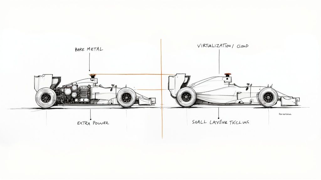
Picture a high-performance pit crew during a race. Every single member has a critical, well-defined job, and they all share one goal: get the car back on the track safely and quickly. The person changing the tires is just as responsible for the outcome as the person refueling the car. A mistake by anyone jeopardizes the entire team. That's the DevOps approach to quality—it's not one person's job, it's everyone's.

From Silos to Shared Ownership

This cultural overhaul completely redefines the role of the modern QA professional. They are no longer manual testers ticking off checklists in a test management tool. Instead, they become quality enablers, coaches, and automation architects.

Their primary technical function shifts to building the test automation frameworks, CI/CD pipeline configurations, and observability dashboards that empower developers to test their own code continuously and effectively. This is the heart of the "shift-left" philosophy—integrating quality activities as early as possible into the development process, often directly within the developer's IDE and the CI pipeline.

The business impact of this is huge. The data doesn't lie: a staggering 99% of organizations that adopt DevOps report positive operational improvements. Digging deeper, 61% specifically point to higher quality deliverables, drawing a straight line from this cultural change to a better product.

DevOps QA isn't about testing more; it's about building a system where quality is an intrinsic, automated part of the delivery pipeline, enabling faster, more confident releases.

This approach transforms the entire software development lifecycle. You can learn more about the principles that drive this change by understanding the core DevOps methodology. The ultimate goal is to create a tight, rapid feedback loop where defects are found and fixed moments after they're introduced—not weeks or months down the line. This proactive stance is what truly sets modern DevOps quality assurance apart from the old way of doing things.

To see just how different these two worlds are, let's put them side-by-side.

Traditional QA vs DevOps Quality Assurance At a Glance

The table below breaks down the core differences between the old, siloed model and the modern, integrated approach. It highlights the profound changes in timing, responsibility, and overall mindset.

Aspect	Traditional QA	DevOps QA
Timing	A separate phase at the end of the cycle	Continuous, integrated throughout the lifecycle
Responsibility	A dedicated QA team owns quality	The entire team (devs, ops, QA) shares ownership
Goal	Find defects before release (Gatekeeping)	Prevent defects and enable speed (Enabling)
Process	Mostly manual testing, some automation	Heavily automated, focused on "shift-left"
Feedback Loop	Long and slow (weeks or months)	Short and fast (minutes or hours)
Role of QA	Acts as a gatekeeper or validator	Acts as a coach, enabler, and automation expert

As you can see, the move to DevOps QA isn't just an incremental improvement; it’s a complete re-imagining of how quality is achieved. It’s about building quality in, not inspecting it on at the very end.

The Four Pillars of a DevOps QA Strategy

To effectively embed quality into your DevOps lifecycle, your strategy must be built on four core, technical pillars. These aren't just concepts; they represent a fundamental shift in how we write, validate, and deploy software. By implementing these four pillars, you can transition from a reactive, gate-based quality model to a proactive and continuous one.

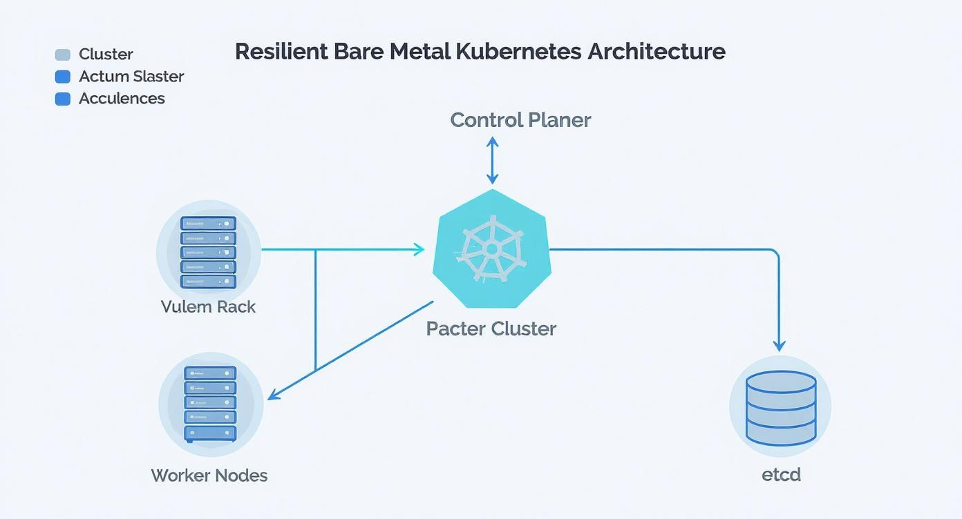
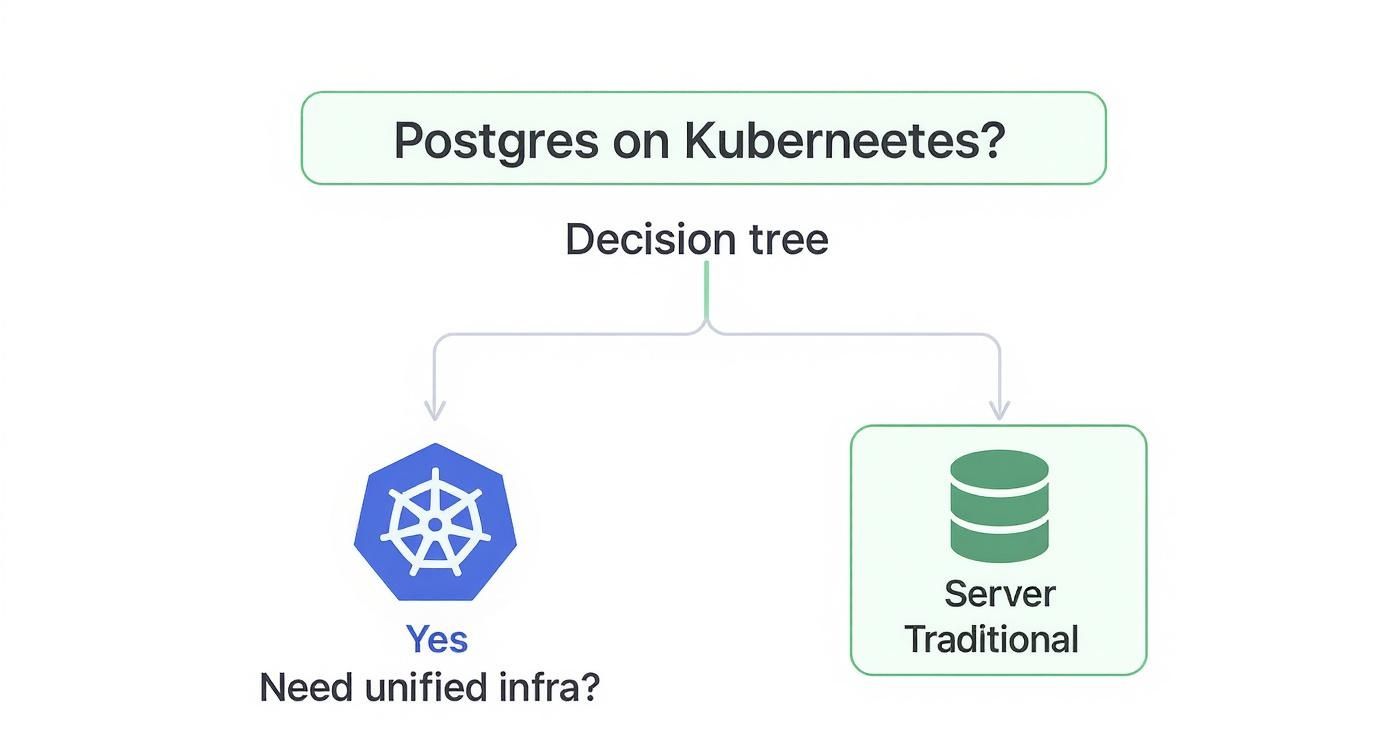
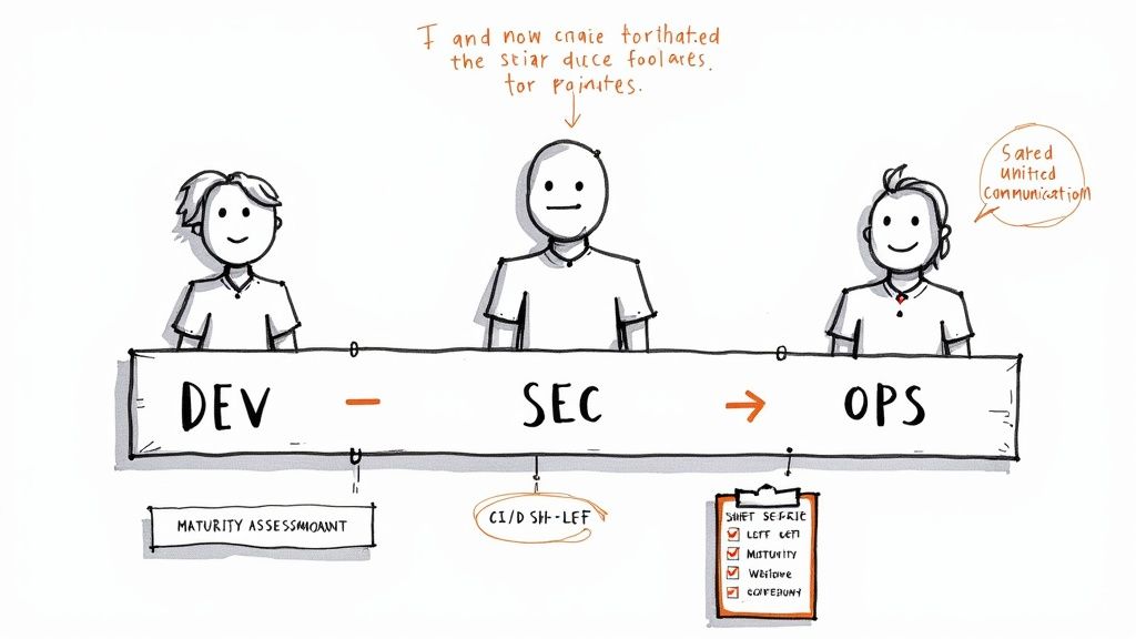
This diagram nails the difference between the old way and the new way. It's all about moving from a siloed, traditional QA model to a DevOps approach grounded in shared responsibility.

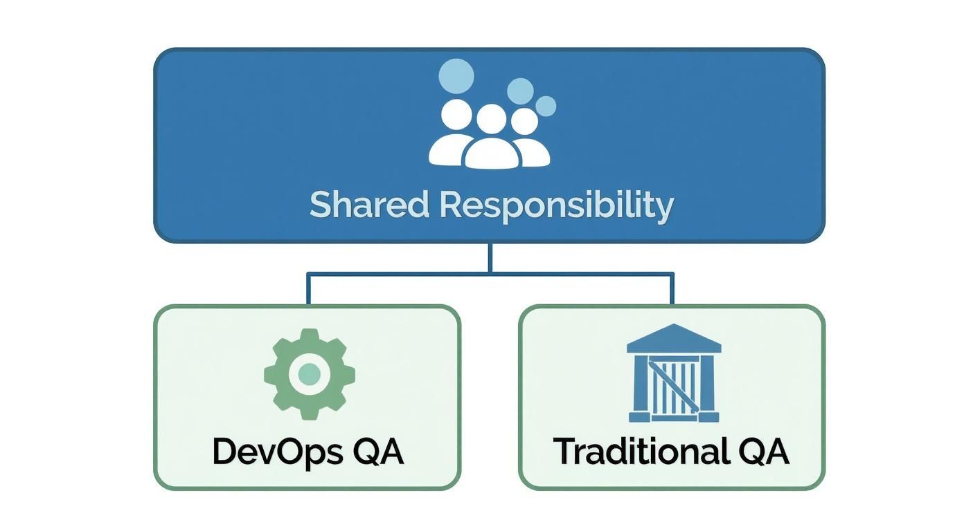
You can see that traditional QA acts as a separate gatekeeper. DevOps QA, on the other hand, is an integrated part of the team’s shared ownership, which makes for a much smoother workflow.

Shifting Left

The first and most powerful pillar is Shifting Left. This is the practice of moving quality assurance activities as early as possible into the development process. Instead of waiting for a feature to be "code complete" before QA sees it, quality becomes part of the development workflow itself.

This means QA professionals get involved during requirements and design, helping define BDD (Behavior-Driven Development) feature files and acceptance criteria. Testers collaborate with developers to design for testability, for example, by ensuring API endpoints are easily mockable or UI components have stable selectors (data-testid attributes).

A concrete technical example is a developer using a static analysis tool like SonarQube integrated directly into their IDE via a plugin. This provides real-time feedback on code quality, security vulnerabilities (e.g., SQL injection risks), and code smells as they type. That immediate feedback is exponentially cheaper and faster than discovering the same issue in a staging environment weeks later. To really get a handle on this concept, check out our deep dive on what is shift left testing.

Continuous Testing

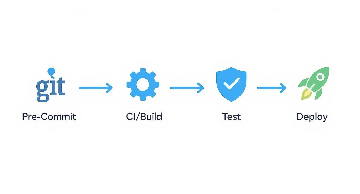
The second pillar, Continuous Testing, is the automated engine that drives a modern DevOps QA strategy. It involves executing automated tests as a mandatory part of the CI/CD pipeline. Every git push triggers an automated sequence of builds and tests, providing immediate feedback on the health of the codebase.

This doesn't mean running a 4-hour E2E test suite on every commit. The key is to layer tests strategically throughout the pipeline to balance feedback speed with test coverage. A typical pipeline might look like this:

• On Commit: The pipeline runs lightning-fast unit tests (go test ./...), linters (eslint .), and static analysis scans. Feedback in < 2 minutes.
• On Pull Request: Broader integration tests are executed, often using Docker Compose to spin up the application and its database dependency. This ensures new code integrates correctly. Feedback in < 10 minutes.
• Post-Merge/Nightly: Slower, more comprehensive end-to-end and performance tests run against a persistent, fully-deployed staging environment.

This constant validation loop catches regressions moments after they’re introduced, preventing them from propagating downstream where they become significantly harder to debug and resolve.

Continuous Testing transforms quality from a distinct, scheduled event into an ongoing, automated process that runs in parallel with development. No build moves forward with known regressions.

Smart Test Automation

Building on continuous testing, our third pillar is Smart Test Automation. This is about more than just writing test scripts; it's about architecting a resilient, maintainable, and valuable test suite. The guiding principle here is the Test Automation Pyramid.

The pyramid advocates for a large base of fast, isolated unit tests, a smaller middle layer of integration tests that validate interactions between components (e.g., service-to-database), and a very small top layer of slow, often brittle end-to-end (E2E) UI tests. Adhering to this model results in a test suite that is fast, reliable, and cost-effective to maintain.

For example, instead of writing dozens of E2E tests that simulate a user logging in through the UI, you'd have one or two critical-path UI tests. The vast majority of authentication logic would be covered by much faster and more stable API-level and unit tests that can be run in parallel.

Infrastructure as Code Validation

The final pillar addresses a common source of production failures: environmental discrepancies. Infrastructure as Code (IaC) Validation is the practice of applying software testing principles to the code that defines your infrastructure—whether it's written in Terraform, Ansible, or CloudFormation.

Just like application code, your IaC must be linted, validated, and tested. Without this, "environment drift" occurs, where dev, staging, and production environments diverge, causing deployments to fail unpredictably.

Tools like Terratest (for Terraform) or InSpec allow you to write automated tests for your infrastructure. A simple Terratest script written in Go might:

1. Execute terraform apply to provision a temporary AWS S3 bucket.
2. Use the AWS SDK to verify the bucket was created with the correct encryption and tagging policies.
3. Check that the associated security group was created with the correct ingress/egress rules.
4. Execute terraform destroy to tear down all resources, ensuring a clean state.

By validating your IaC, you guarantee that every environment is provisioned identically and correctly, providing a stable, reliable foundation for your application deployments.

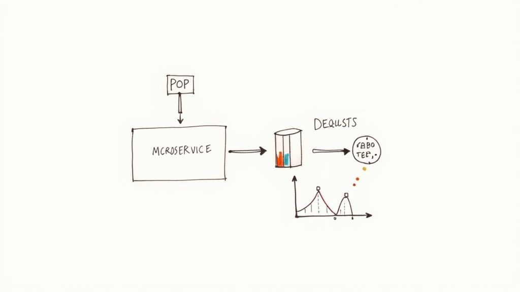
Building an Integrated DevOps QA Toolchain

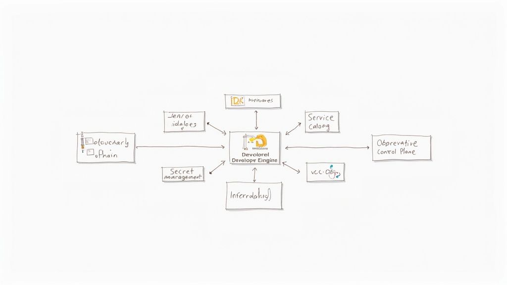
An effective DevOps quality assurance strategy is powered by a well-integrated collection of tools working in concert. This toolchain is the technical backbone of your CI/CD pipeline, automating the entire workflow from a git commit to a validated feature running in production. A disjointed set of tools creates friction, slows down feedback, and undermines the velocity you're striving for.

Conversely, a seamless toolchain acts as a "quality nervous system." An event in one part of the system—like a GitHub pull request—instantly triggers a reaction in another, like a Jenkins pipeline run. The goal is to create an automated, observable, and reliable path to production where quality checks are embedded, not bolted on.

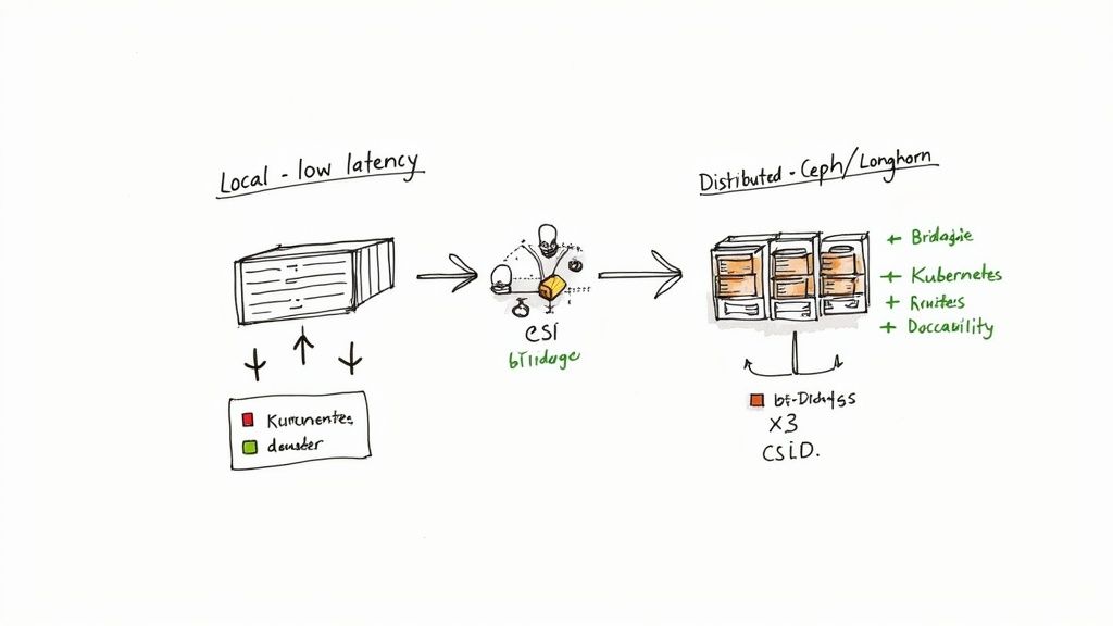
This diagram gives a great high-level view of how a CI/CD pipeline brings different tools together to automate both testing and monitoring.

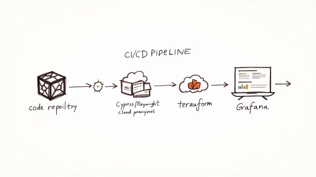
You can see how code moves from the repository through various automated stages, with observability tools providing a constant feedback loop.

Key Components of a Modern QA Toolchain

To build this kind of integrated system, you need specific tools for each stage of the lifecycle. A solid DevOps QA toolchain depends heavily on automation, and understanding the overarching benefits of workflow automation can make it much easier to justify investing in the right tools.

• CI/CD Orchestrators: These are the pipeline engines. Tools like Jenkins, GitLab CI, or GitHub Actions execute declarative pipeline definitions (e.g., Jenkinsfile, .gitlab-ci.yml, .github/workflows/main.yml) to build, test, and deploy applications.

• Testing Frameworks: This is where validation logic lives. You have frameworks like Cypress or Playwright for robust end-to-end browser automation. For unit and integration tests, you’ll use language-specific tools like JUnit for Java or Pytest for Python.

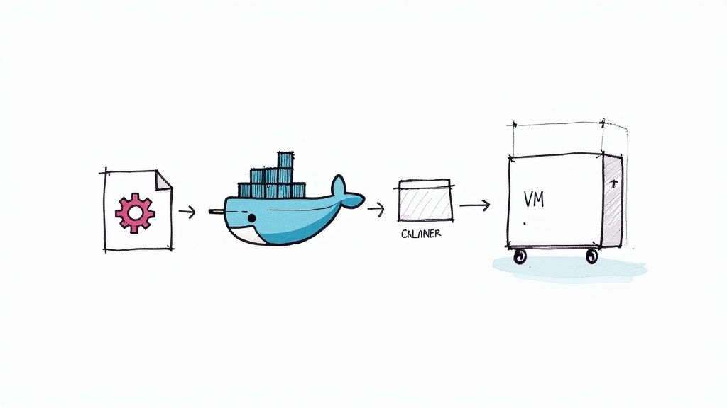
• Containerization and IaC: Tools like Docker are non-negotiable for creating consistent, portable application environments. Infrastructure is defined as code using tools like Terraform, which guarantees that dev, staging, and prod environments are identical and reproducible.

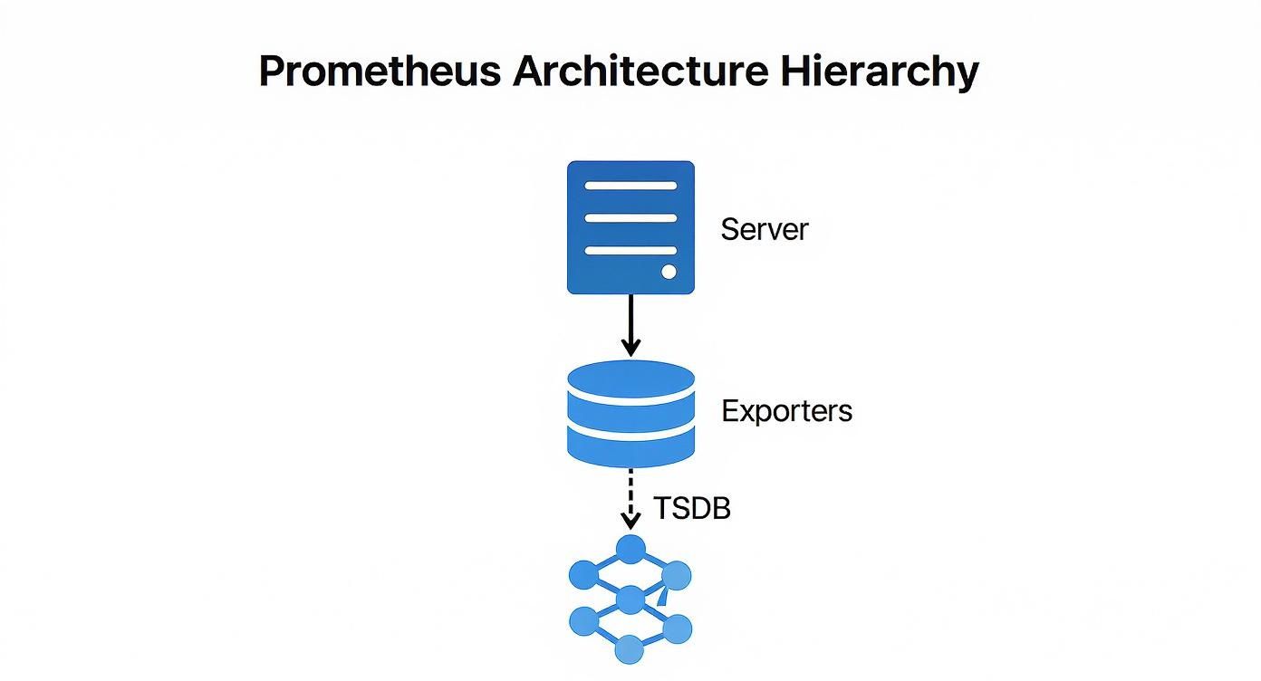
• Observability Platforms: Post-deployment, you need visibility into application behavior. This is where tools like Prometheus scrape metrics, logs are aggregated (e.g., with the ELK stack), and Grafana provides visualization dashboards, giving real-time insight into performance and health.

Weaving the Tools Together in Practice

The real power is unleashed when these tools are integrated into a cohesive workflow. Automated testing has become a cornerstone of modern DevOps QA, with nearly 85% of organizations globally using it to improve software quality. This isn't just a trend; it's a fundamental shift in how teams manage quality.

Let's walk through a technical example using GitHub Actions. When a developer opens a pull request, the .github/workflows/ci.yml file triggers the pipeline:

1. Build Stage: A workflow job checks out the code, sets up the required language environment (e.g., Node.js), and runs npm run build to compile the application. The resulting artifacts are uploaded for later stages.
2. Test Stage: A separate job, often running in parallel, uses docker-compose up to launch the application and a test database. It then executes a suite of Playwright E2E tests against the ephemeral environment. Test results (e.g., JUnit XML reports) are published. To get this step right, it’s critical to properly automate your software testing.
3. Deploy Stage: If tests pass and the PR is merged to main, a separate workflow triggers. This job uses Terraform Cloud credentials to run terraform apply, deploying the new application version to a staging environment on AWS.
4. Monitoring Feedback: The application, running in its Terraform-managed environment, is already configured with a Prometheus client library to expose metrics on a /metrics endpoint. A Prometheus server scrapes this endpoint, and any anomalies (e.g., increased HTTP 500 errors) trigger an alert in Alertmanager, closing the feedback loop.

This flow is what a true DevOps quality assurance process looks like in action. Quality isn't just checked at a single gate; it's validated continuously through an automated, interconnected toolchain that gives you fast, reliable feedback every step of the way.

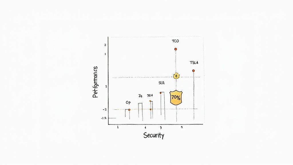
Measuring the Success of Your DevOps QA

If you’re not measuring, you’re just guessing. In DevOps quality assurance, metrics are not vanity numbers for a report; they are critical signals indicating the health of your delivery pipeline. Tracking the right key performance indicators (KPIs) allows you to make data-driven decisions to optimize your processes.

This is about moving beyond vanity metrics—like lines of code written or the raw number of tests run—and focusing on KPIs that directly measure your pipeline's velocity, stability, and production quality.

Gauging Pipeline Velocity and Resilience

A successful DevOps practice is built on two pillars: how fast you can deliver value and how quickly you can recover from failure. The DORA metrics are the industry standard for measuring this.

Mean Time to Recovery (MTTR) is arguably the most critical metric for operational stability. It measures the average time from a production failure detection to full restoration of service. A low MTTR is the hallmark of a resilient system with mature observability and incident response practices.

To improve MTTR, implement these technical solutions:

• Structured Logging & Alerting: Ensure your applications output structured logs (e.g., JSON) and have robust alerting rules in Prometheus/Alertmanager to detect issues proactively.
• Automated Rollbacks: Design your deployment pipeline with a one-click or automated rollback capability. For example, a canary deployment that fails health checks should automatically roll back to the previous stable version.
• Chaos Engineering: Use tools like Gremlin to intentionally inject failures (e.g., network latency, pod termination) into your staging environment to practice and harden your incident response.

Another key DORA metric is Deployment Frequency. This measures how often your organization successfully releases to production. High-performing teams deploy on-demand, often multiple times per day, signaling a highly automated, low-risk delivery process.

Tracking Production Quality and User Impact

Ultimately, DevOps QA aims to deliver a reliable product to customers. These metrics directly reflect the impact of your quality efforts on the end-user experience.

The Defect Escape Rate measures the percentage of bugs discovered in production rather than during the pre-release testing phases. A high rate indicates that your automated test coverage has significant gaps or that your shift-left strategy is ineffective.

A rising Defect Escape Rate is a serious warning sign. It tells you that your automated test suites have blind spots or your manual exploratory testing isn’t focused on the right areas. This directly erodes user trust and damages your brand's reputation.

The Change Failure Rate is the percentage of deployments to production that result in a degraded service and require remediation (e.g., a rollback, hotfix). Elite DevOps teams maintain a change failure rate below 15%. A high rate points to inadequate testing, unstable infrastructure, or a flawed release process.

To truly understand your quality posture, you need to track a combination of these metrics. Here’s a quick breakdown of the essentials:

Essential DevOps QA Metrics

Metric	Definition	What It Measures
Mean Time to Recovery (MTTR)	The average time it takes to restore service after a production failure.	The resilience and stability of your system and the effectiveness of your incident response.
Deployment Frequency	How often code is deployed to production.	The speed and efficiency of your delivery pipeline. A higher frequency suggests a more mature process.
Defect Escape Rate	The percentage of defects discovered in production instead of pre-release testing.	The effectiveness of your "shift-left" testing and overall quality gates.
Change Failure Rate	The percentage of deployments that result in a production failure.	The quality of your release process and the stability of your code and infrastructure.
Automated Test Pass Rate	The percentage of automated tests that pass on a given run.	The health and reliability of your test suite itself. A low rate can indicate "flaky" tests.

Tracking these KPIs provides a holistic view, moving you from simply measuring activity to understanding the real-world impact of your quality initiatives.

Evaluating Test Efficacy and Process Health

It's easy to get caught up in the numbers, but not all tests are created equal. You need to measure the effectiveness of your testing strategy and the health of your automation to ensure your pipeline remains trustworthy.

A common pitfall is chasing 100% Code Coverage. While a useful indicator, it's often a vanity metric. A test suite can achieve high coverage by touching every line of code without asserting any meaningful business logic. A better approach is focusing on Critical Path Coverage, ensuring that your most important user journeys and business-critical API endpoints are thoroughly tested.

Finally, rigorously monitor your Automated Test Pass Rate. A consistently low rate often indicates "flaky tests"—tests that fail intermittently due to factors like network latency or race conditions, not actual code defects. Flaky tests are toxic because they erode developer trust in the CI pipeline, leading them to ignore legitimate failures. Actively identify, quarantine, and fix flaky tests to maintain a reliable and fast feedback loop.

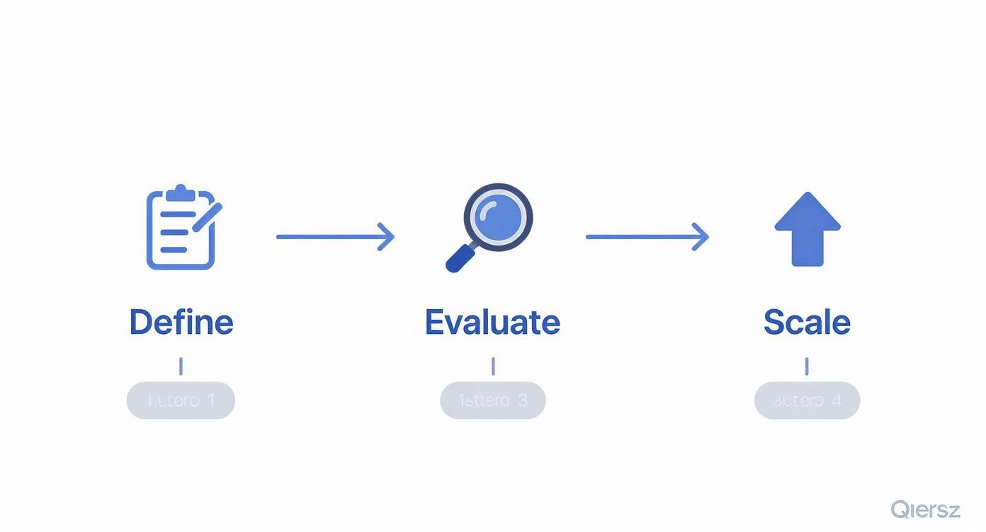
Your Roadmap to Implementing DevOps QA

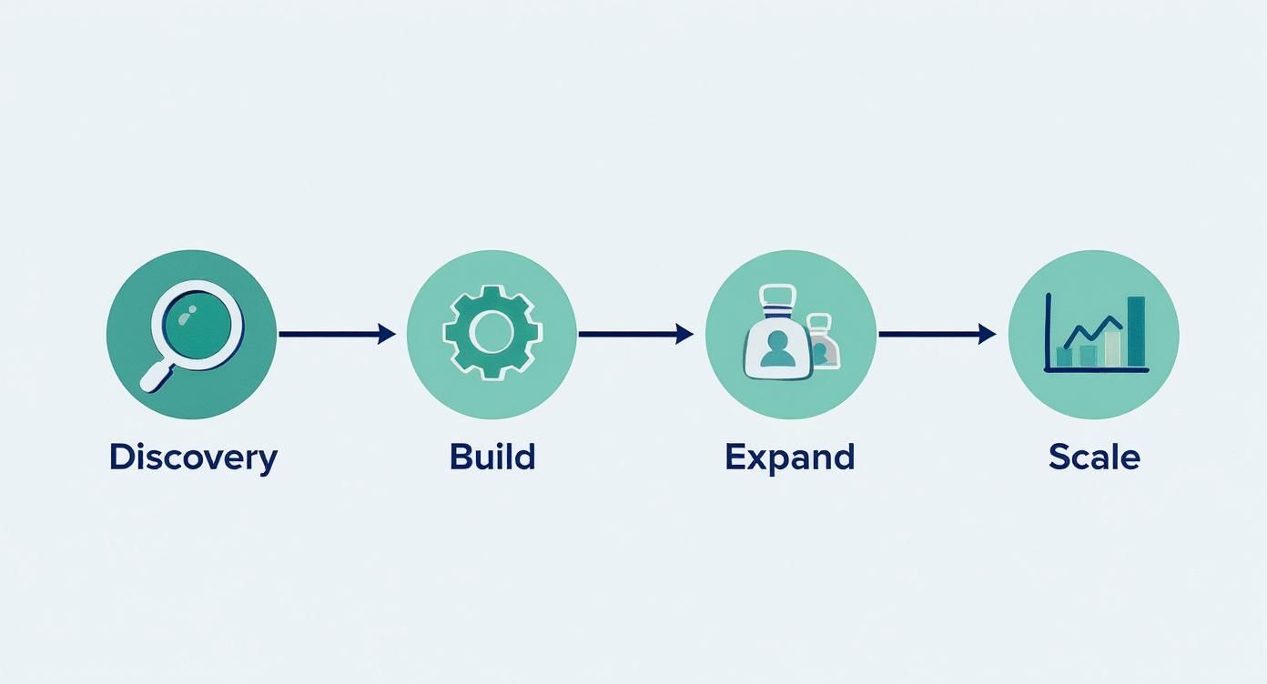
Transitioning to a mature DevOps QA practice is a strategic, iterative process. You need a clear, phased roadmap that builds momentum without disrupting current delivery cycles. This roadmap provides a technical blueprint, guiding you from assessment to continuous optimization.

Phase 1: Baseline and Assess

Before you can engineer a better process, you must quantify your current state. This phase is about discovery and data collection. The goal is to create a data-driven, objective assessment of your existing workflows, toolchains, and team capabilities.

Start by mapping your entire software delivery value stream, from idea to production. Identify manual handoffs, long feedback loops, and testing bottlenecks. This is a technical audit, not just a process review.

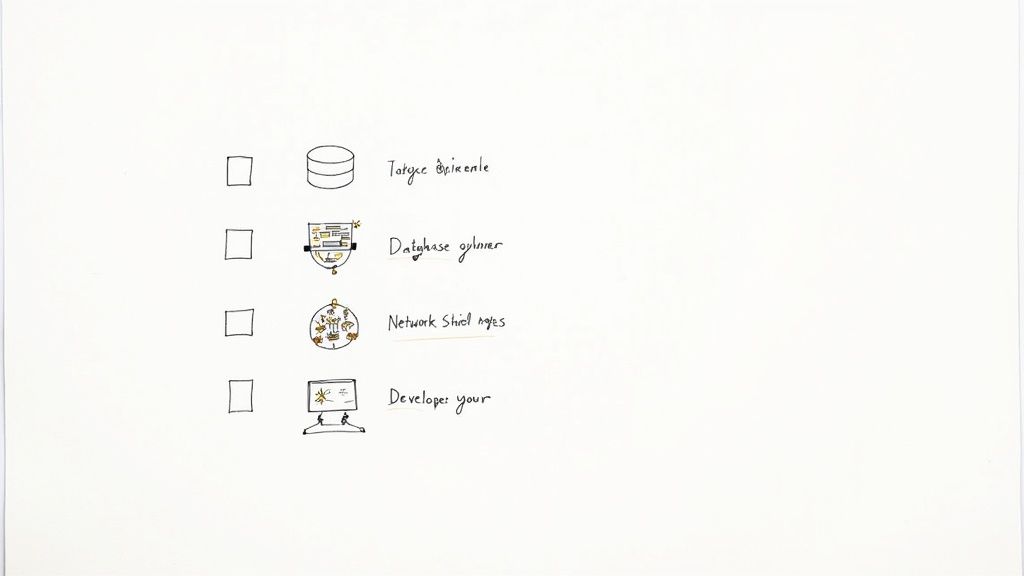
Your Practical Checklist:

• Audit Your Toolchain: Document every tool for version control (Git provider), CI/CD (Jenkins, GitLab CI), testing (frameworks, runners), and observability (monitoring, logging). Identify integration gaps.
• Analyze Key Metrics: Instrument your pipelines to collect baseline DORA metrics: Deployment Frequency, Change Failure Rate, and Mean Time to Recovery (MTTR). This is your "before" state.
• Interview Your Teams: Conduct structured interviews with developers, QA engineers, and SREs. Identify specific technical friction points (e.g., "Our E2E test suite takes 2 hours to run locally").

Phase 2: Pilot and Prove

With a clear baseline, select a single pilot project to demonstrate the value of DevOps QA. A "big bang" approach is doomed to fail due to organizational inertia. Instead, choose one high-impact, low-risk project to build early momentum and create internal champions.

This pilot serves as your proof-of-concept. A good candidate is a new microservice or a well-contained component of a monolith where you can implement a full CI/CD pipeline with integrated testing.

The success of your pilot project is your internal marketing campaign. It provides the concrete evidence needed to secure buy-in from leadership and inspire other teams to adopt new practices.

The focus here is on a measurable "quick win." For example, demonstrate that integrating automated tests into the CI pipeline reduced the regression testing cycle for the pilot component from 3 days to 15 minutes.

Phase 3: Standardize and Scale

With a successful pilot, it's time to scale what you've learned. This phase is about standardizing the tools, frameworks, and pipeline patterns that proved effective. You are creating a "paved road"—a set of repeatable, well-supported blueprints that enable other teams to adopt best practices easily.

This involves building reusable infrastructure and sharing knowledge, not just writing documents.

Your Practical Checklist:

• Establish a Toolchain Standard: Officially adopt and support a primary toolchain based on the pilot's success (e.g., GitLab CI, Cypress, Terraform).
• Create Reusable Pipeline Templates: Build CI/CD pipeline templates (e.g., GitLab CI includes, GitHub Actions reusable workflows) that other teams can import and extend. This ensures consistent quality gates across the organization.
• Develop a Center of Excellence: Form a small, dedicated team of experts to act as internal consultants. Their role is to help other teams adopt the standard toolchain and overcome technical hurdles.

Phase 4: Optimize and Innovate

You've built a scalable foundation. Now the goal is continuous improvement. This phase involves moving beyond defect detection to defect prevention and system resilience. The focus shifts from simply catching bugs to building systems that are inherently more robust.

This is where you introduce advanced techniques like chaos engineering (e.g., using LitmusChaos) to proactively test system resilience or performance testing as a continuous, automated stage in the pipeline (e.g., using k6). AI is also becoming a critical enabler; an incredible 60% of organizations now use AI in their QA processes, a figure that doubled in just one year. This includes AI-powered test generation, visual regression testing, and anomaly detection in observability data. You can dig into more insights like this over on DevOps Digest.

By embracing these advanced practices, you transform quality from a cost center into a true competitive advantage, enabling you to innovate with both speed and confidence.

Frequently Asked Questions About DevOps QA

As organizations implement DevOps quality assurance, common and highly technical questions arise. The shift from traditional, siloed QA to an integrated model fundamentally alters roles, workflows, and team structures. Here are the answers to the most frequent technical questions.

What Is the Role of a QA Engineer in a DevOps Culture

In a mature DevOps culture, the QA Engineer role evolves from a manual tester to a Software Development Engineer in Test (SDET) or Quality Engineer. They are no longer a separate gatekeeper but a "quality coach" and automation architect embedded within the development team.

Their primary technical responsibilities shift to:

• Building Test Automation Frameworks: They design, build, and maintain the core test automation frameworks (e.g., a Cypress or Playwright framework with custom commands and page objects) that developers use.
• CI/CD Pipeline Integration: They are experts in configuring CI/CD pipelines (e.g., writing YAML for GitHub Actions or Jenkinsfiles) to integrate various testing stages (unit, integration, E2E) effectively.
• Observability and Monitoring: They work with SREs to define quality-centric monitoring and alerting. They help create dashboards in Grafana to track metrics like error rates, latency, and defect escape rates.

Their goal is to make quality a shared, automated, and observable attribute of the software delivery process, owned by the entire team.

How Do You Handle Manual and Exploratory Testing in DevOps

Automation is the core of DevOps QA, but it does not eliminate the need for manual and exploratory testing. Automation is excellent for verifying known requirements and preventing regressions. It is poor at discovering novel bugs or evaluating subjective user experience.

That's where human expertise remains critical. Exploratory testing is essential for investigating complex user workflows, assessing usability, and identifying edge cases that automated scripts would miss.

The technical approach is to integrate it strategically:

• Automate all deterministic, repetitive regression checks and execute them in the CI pipeline.
• Use feature flags to deploy new functionality to a limited audience or internal users for "dogfooding" and exploratory testing in a production-like environment.
• Conduct time-boxed exploratory testing sessions on new, complex features before a full production rollout.

This hybrid approach provides the speed of automation with the depth of human-driven exploration.

Manual testing isn't the enemy of DevOps; it's a strategic partner. You automate the predictable so that your human experts can focus their creativity on exploring the unpredictable. That's how you achieve real coverage.

Can You Fully Eliminate a Separate QA Team

While the goal is to eliminate the silo between development and QA, most high-performing organizations do not eliminate quality specialists entirely. Instead, the centralized QA team's function evolves.

They transform from a hands-on testing service into a Center of Excellence (CoE) or Platform Team. This centralized group is not responsible for the day-to-day testing of product features. Instead, their technical mandate is to:

• Define and maintain the standard testing toolchains, frameworks, and libraries for the entire organization.
• Build and support reusable CI/CD pipeline components (e.g., shared Docker images, pipeline templates) that enforce quality gates.
• Provide expert consultation, training, and support to the embedded Quality Engineers and developers within product teams.

This model provides organizational consistency and economies of scale while embedding the day-to-day ownership of quality directly within the teams that build the software.

---

Ready to accelerate your software delivery and improve reliability? The experts at OpsMoon can help you build a world-class DevOps QA strategy. We connect you with the top 0.7% of global engineering talent to assess your maturity, design a clear roadmap, and implement the toolchains and processes you need to succeed. Start with a free work planning session today.

Deploying Kubernetes on bare metal means installing the container orchestrator directly onto physical servers without an intermediary hypervisor layer. This direct hardware access eliminates virtualization overhead, giving applications raw, unfiltered access to the server's compute, memory, I/O, and networking resources.

The result is maximum performance and the lowest possible latency, a critical advantage for high-throughput workloads like databases, message queues, AI/ML training, and high-frequency trading platforms. This guide provides a technical deep-dive into the architecture and operational practices required to build and maintain a production-grade bare metal Kubernetes cluster.

Why Choose Kubernetes on Bare Metal

When an engineering team decides where to run their Kubernetes clusters, they're usually weighing three options: cloud-managed services like GKE or EKS, virtualized on-prem environments, or bare metal. Cloud and VMs offer operational convenience, but a Kubernetes bare metal setup is engineered for raw performance.

Think of it as the difference between a production race car and a road-legal supercar. Running Kubernetes on bare metal is like bolting the engine directly to the chassis—every joule of energy translates to speed with zero waste. Virtualization introduces a complex transmission and comfort features; it works, but that abstraction layer consumes resources and introduces I/O latency, measurably degrading raw performance.

To quantify this, here’s a technical breakdown of how these models compare.

Kubernetes Deployment Models at a Glance

Deployment Model	Performance & Latency	Cost Model	Operational Overhead
Bare Metal	Highest; direct hardware access, no hypervisor tax.	Best for stable workloads (CapEx); predictable TCO.	High; requires deep expertise in hardware, networking, and OS management.
Virtualized	Good; ~5-15% CPU/memory overhead from hypervisor.	Moderate; software licensing (e.g., vSphere) adds to CapEx.	Medium; hypervisor abstracts hardware management.
Cloud-Managed	Good; provider-dependent, "noisy neighbor" potential.	Lowest for variable workloads (OpEx); pay-as-you-go.	Low; managed by cloud provider.

This table gives you a starting point, but the "why" behind choosing bare metal goes much deeper.

The Core Drivers for Bare Metal

The decision to eliminate the hypervisor is a strategic one, driven by specific technical and business requirements where performance and control outweigh the convenience of managed services.

The primary technical justifications are:

• Unmatched Performance: Bypassing the hypervisor grants applications direct access to CPU scheduling, physical RAM, and network interface cards (NICs). This slashes I/O latency and eliminates the "hypervisor tax"—the CPU and memory overhead consumed by the virtualization software itself. Workloads that are sensitive to jitter, such as real-time data processing, benefit immensely.
• Predictable Cost Structure: Bare metal shifts infrastructure spending from a variable, operational expense (OpEx) model to a more predictable capital expense (CapEx) model. For stable, long-running workloads, owning the hardware can dramatically lower the Total Cost of Ownership (TCO) compared to the recurring fees of cloud services.
• Complete Infrastructure Control: Self-hosting provides total autonomy over the entire stack. You control server firmware versions, kernel parameters, network topology (e.g., L2/L3 fabric), and storage configurations. This level of control is essential for specialized use cases or strict regulatory compliance.

A Growing Industry Standard

This is no longer a niche strategy. The global developer community has standardized on Kubernetes, with 5.6 million developers now using the platform. As Kubernetes solidifies its position with a massive 92% market share of container orchestration tools, more organizations are turning to bare metal to extract maximum value from their critical applications. Read more about the rise of bare metal Kubernetes adoption.

By removing abstraction layers, a bare metal Kubernetes setup empowers teams to fine-tune every component for maximum efficiency. This level of control is essential for industries like high-frequency trading, real-time data processing, and large-scale AI/ML model training, where every microsecond counts.

Ultimately, choosing a bare metal deployment is about making a deliberate trade-off. You accept greater operational responsibility in exchange for unparalleled performance, cost-efficiency, and total control. This guide will provide the technical details required to build, manage, and scale such an environment.

Designing a Resilient Bare Metal Architecture

Building a resilient Kubernetes bare metal cluster is an exercise in distributed systems engineering. You are not just configuring software; you are designing a fault-tolerant system from the physical layer up. Every decision—from server specifications to control plane topology—directly impacts the stability and performance of the entire platform.

The first step is defining the role of each physical machine. A production Kubernetes cluster consists of two primary node types: control plane nodes, which run the Kubernetes API server, scheduler, and controller manager, and worker nodes, which execute application pods. High availability (HA) is non-negotiable for production, meaning you must eliminate single points of failure.

A minimal production-grade topology consists of three control plane nodes and at least three worker nodes. To achieve true fault tolerance, these servers must be distributed across different physical failure domains: separate server racks, power distribution units (PDUs), and top-of-rack (ToR) switches. This ensures that the failure of a single physical component does not cause a cascading cluster outage.

Control Plane and etcd Topology

A critical architectural decision is the placement of etcd, the consistent and highly-available key-value store that holds all Kubernetes cluster state. If etcd loses quorum, your cluster is non-functional. For HA, there are two primary topologies.

• Stacked Control Plane (etcd on control plane nodes): This is the most common and resource-efficient approach. The etcd members run directly on the same machines as the Kubernetes control plane components. It's simpler to configure and requires fewer servers.
• External etcd Cluster (etcd on dedicated nodes): In this model, etcd is deployed on a dedicated cluster of servers, completely separate from the Kubernetes control plane. While it requires more hardware and operational complexity, it provides maximum isolation. An issue on an API server (e.g., a memory leak) cannot impact etcd performance, and vice-versa.

For most bare metal deployments, a stacked control plane offers the best balance of resilience and operational simplicity. However, for extremely large-scale or mission-critical clusters where maximum component isolation is paramount, an external etcd cluster provides an additional layer of fault tolerance.

Sizing Your Bare Metal Nodes

Hardware selection must be tailored to the specific role each node will play. A generic server specification is insufficient for a high-performance cluster. The hardware profile must match the workload.

Here is a baseline technical specification guide for different node roles.

Node Type	Workload Example	CPU Recommendation	RAM Recommendation	Storage Recommendation
Control Plane	Kubernetes API, etcd	8-16 Cores	32-64 GB DDR4/5	Critical: High IOPS, low-latency NVMe SSDs for etcd data directory (/var/lib/etcd)
Worker (General)	Web Apps, APIs	16-32 Cores	64-128 GB	Mixed SSD/NVMe for fast container image pulls and local storage
Worker (Compute)	AI/ML, Data Proc.	64+ Cores (w/ GPU)	256-512+ GB	High-throughput RAID 0 NVMe array for scratch space
Worker (Storage)	Distributed DBs (e.g., Ceph)	32-64 Cores	128-256 GB	Multiple large capacity NVMe/SSDs for distributed storage pool

These specifications are not arbitrary. A control plane node's performance is bottlenecked by etcd's disk I/O. A 2023 industry survey found that over 45% of performance issues in self-managed clusters were traced directly to insufficient I/O performance for the etcd data store. Using enterprise-grade NVMe drives for etcd is a hard requirement for production.

When you thoughtfully plan out your node roles and etcd layout, you're not just racking servers—you're building a cohesive, fault-tolerant platform. This upfront design work pays off massively down the road by preventing cascading failures and making it way easier to scale. It’s the true bedrock of a solid bare metal strategy.

Solving Bare Metal Networking Challenges

In a cloud environment, networking is highly abstracted. Requesting a LoadBalancer service results in the cloud provider provisioning and configuring an external load balancer automatically.

On bare metal Kubernetes, this abstraction vanishes. You are responsible for the entire network stack, from the physical switches and routing protocols to the pod-to-pod communication overlay.

This control is a primary reason for choosing bare metal, but it necessitates a robust networking strategy. You must select, configure, and manage two key components: a load balancing solution for north-south traffic (external to internal) and a Container Network Interface (CNI) plugin for east-west traffic (pod-to-pod).

This diagram shows how the control plane, worker nodes, and etcd form the core of a resilient bare metal setup. Your networking layer is the glue that holds all of this together.

You can see how each piece has a distinct role, which underscores just how critical it is to have a networking fabric that reliably connects them all.

Exposing Services with MetalLB

To replicate the functionality of a cloud LoadBalancer service on-premises, MetalLB has become the de facto standard. It integrates with your physical network to assign external IP addresses to Kubernetes services from a predefined pool.

MetalLB operates in two primary modes:

1. Layer 2 (L2) Mode: The simplest configuration. A single node in the cluster announces the service IP address on the local network using Address Resolution Protocol (ARP). If that node fails, another node takes over the announcement. While simple, it creates a performance bottleneck as all traffic for that service is funneled through the single leader node. It is suitable for development or low-throughput services.

2. BGP Mode: The production-grade solution. MetalLB establishes a Border Gateway Protocol (BGP) peering session with your physical network routers (e.g., ToR switches). This allows MetalLB to advertise the service IP to the routers, which can then use Equal-Cost Multi-Path (ECMP) routing to load-balance traffic across multiple nodes running the service pods. This provides true high availability and scalability, eliminating single points of failure.

The choice between L2 and BGP is a choice between simplicity and production-readiness. L2 is excellent for lab environments. For any production workload, implementing BGP is essential to achieve the performance and fault tolerance expected from a bare metal deployment.

Selecting the Right CNI Plugin

While MetalLB handles external traffic, the Container Network Interface (CNI) plugin manages pod-to-pod networking within the cluster. CNI choice is critical to performance, with bare metal clusters often achieving network latency up to three times lower than typical virtualized environments.

Here is a technical comparison of leading CNI plugins:

CNI Plugin	Key Technology	Best For
Calico	BGP for routing, iptables/eBPF for policy	Performance-critical applications and secure environments requiring granular network policies. Its native BGP mode integrates seamlessly with MetalLB for a unified routing plane.
Cilium	eBPF (extended Berkeley Packet Filter)	Modern, high-performance clusters requiring deep network observability, API-aware security, and service mesh capabilities without a sidecar.
Flannel	VXLAN overlay	Simple, quick-start deployments where advanced network policies are not an immediate requirement. It's easy to configure but introduces encapsulation overhead.

For most high-performance bare metal clusters, Calico is an excellent choice due to its direct BGP integration. However, Cilium is rapidly gaining traction by leveraging eBPF to implement networking, observability, and security directly in the Linux kernel, bypassing slower legacy paths like iptables for superior performance. To see how these ideas play out in other parts of the ecosystem, check out our deep dive on service meshes like Linkerd vs Istio.

Mastering Storage for Stateful Applications

Stateless applications are simple, but business-critical workloads—databases, message queues, AI/ML models—are stateful. They require persistent storage that outlives any individual pod. On Kubernetes on bare metal, you cannot provision a block storage volume with a simple API call; you must engineer a robust storage solution yourself.

The Container Storage Interface (CSI) is the standard API that decouples Kubernetes from specific storage systems. It acts as a universal translation layer, allowing Kubernetes to provision, attach, and manage volumes from any CSI-compliant storage backend, whether it's a local NVMe drive or a distributed filesystem.

The Role of PersistentVolumes and Claims

Storage is exposed to applications through two core Kubernetes objects:

• PersistentVolume (PV): A cluster-level resource representing a piece of physical storage. It is provisioned by an administrator or dynamically by a CSI driver.
• PersistentVolumeClaim (PVC): A namespaced request for storage by a pod. A developer can request spec.resources.requests.storage: 10Gi with a specific storageClassName without needing to know the underlying storage technology.

The CSI driver acts as the controller that satisfies a PVC by provisioning a PV from its backend storage pool. This process, known as "dynamic provisioning," is essential for scalable, automated storage management.

Choosing Your Bare Metal Storage Strategy

Your storage architecture directly impacts application performance, resilience, and scalability. There are two primary strategies, each suited for different workload profiles.

The optimal storage solution is not one-size-fits-all. It's about matching the storage technology's performance and resilience characteristics to the specific I/O requirements of the application.

1. Local Storage for Maximum Performance

For workloads where latency is the primary concern, nothing surpasses direct-attached local storage (NVMe or SSD).

The Local Path Provisioner is a lightweight CSI driver that exposes host directories as storage. It's simple, fast, and provides direct access to the underlying drive's performance. When a PVC is created, the provisioner finds a node with sufficient capacity and binds the PVC to a PV representing a path on that node's filesystem (e.g., /mnt/disks/ssd1/pvc-xyz).

The trade-off is that the data is tied to a single node. If the node fails, the data is lost. This makes local storage ideal for replicated databases (where the application handles redundancy), cache servers, or CI/CD build jobs.

2. Distributed Storage for Resilience and Scale

For mission-critical stateful applications that cannot tolerate data loss, a distributed storage system is required. These solutions pool the storage from multiple nodes into a single, fault-tolerant, software-defined storage layer.

Two leading open-source options are:

• Rook with Ceph: Rook is a Kubernetes operator that automates the deployment and management of Ceph, a powerful, scalable, and versatile distributed storage system. Ceph can provide block storage (RBD), object storage (S3/Swift compatible), and filesystems (CephFS) from a single unified cluster.
• Longhorn: Developed by Rancher, Longhorn offers a more user-friendly approach to distributed block storage. It automatically replicates volume data across multiple nodes. If a node fails, Longhorn automatically re-replicates the data to a healthy node, ensuring data availability for the application.

These systems provide data redundancy at the cost of increased network latency due to data replication. They are the standard for databases, message brokers, and any stateful service where data durability is non-negotiable.

Choosing Your Cluster Installer and Provisioner

Bootstrapping a Kubernetes bare metal cluster from scratch is a complex process involving OS installation, package configuration, certificate generation, and component setup on every server.

An ecosystem of installers and provisioners has emerged to automate this process. Your choice of tool will fundamentally shape your cluster's architecture, security posture, and day-to-day operational model. The decision balances flexibility and control against operational simplicity and production-readiness.

Foundational Flexibility with Kubeadm

kubeadm is the official cluster installation toolkit from the Kubernetes project. It is not a complete provisioning solution; it does not install the OS or configure the underlying hardware. Instead, it provides a set of robust command-line tools (kubeadm init, kubeadm join) to bootstrap a best-practice Kubernetes cluster on pre-configured machines.

Kubeadm offers maximum flexibility, allowing you to choose your own container runtime, CNI plugin, and other components.

• Pro: Complete control over every cluster component and configuration parameter.
• Con: You are responsible for all prerequisite tasks, including OS hardening, certificate management, and developing the automation to provision the servers themselves.

This path requires significant in-house expertise and is best suited for teams building a highly customized Kubernetes platform.

Opinionated Distributions for Production Readiness

For a more streamlined path to a production-ready cluster, opinionated distributions bundle Kubernetes with pre-configured, hardened components. They trade some flexibility for enhanced security and operational simplicity out-of-the-box.

These distributions are complete Kubernetes platforms, not just installers. They make critical architectural decisions for you, such as selecting a FIPS-compliant container runtime or implementing a CIS-hardened OS, to deliver a production-grade system from day one.

Choosing the right distribution depends on your specific requirements for security, ease of use, or infrastructure immutability.

Comparison of Bare Metal Kubernetes Installers

This table compares popular tools for bootstrapping and managing Kubernetes clusters on bare metal infrastructure, focusing on key decision-making criteria.

Tool	Primary Use Case	Configuration Method	Security Focus	Ease of Use
Kubeadm	Foundational, flexible cluster creation for teams wanting deep control.	Command-line flags and YAML configuration files.	Follows Kubernetes best practices but relies on user for hardening.	Moderate; requires significant manual setup for OS and infra.
RKE2	High-security, compliant environments (e.g., government, finance).	Simple YAML configuration file.	FIPS 140-2 validated, CIS hardened by default.	High; designed for simplicity and operational ease.
k0s	Lightweight, zero-dependency clusters that are easy to distribute and embed.	Single YAML file or command-line flags.	Secure defaults, with options for FIPS compliance.	Very High; packaged as a single binary for ultimate simplicity.
Talos	Immutable, API-managed infrastructure for GitOps-centric teams.	Declarative YAML managed via an API.	Minimalist, read-only OS; removes SSH and console access.	High, but requires a steep learning curve for its unique model.

RKE2 and k0s provide a traditional system administration experience. Talos represents a paradigm shift, enforcing an immutable, API-driven GitOps model for managing the entire node, not just the Kubernetes layer.

Declarative Provisioning with Cluster API

After initial installation, you need a way to manage the lifecycle of the physical servers themselves. Cluster API (CAPI) is a Kubernetes sub-project that extends the Kubernetes API to manage cluster infrastructure declaratively.

Using a provider like Metal³, CAPI can automate the entire physical server lifecycle: provisioning the OS via PXE boot, installing Kubernetes components, and joining the machine to a cluster. This enables a true GitOps workflow for bare metal. Your entire data center can be defined in YAML files, version-controlled in Git, and reconciled by Kubernetes controllers. For more on this pattern, see our guide on using Terraform with Kubernetes.

Automating Day-Two Operations and Scaling

Provisioning a Kubernetes bare metal cluster is Day One. The real engineering challenge is Day Two: the ongoing management, maintenance, and scaling of the cluster.

Unlike managed cloud services, where these tasks are handled by the provider, a bare metal environment places 100% of this responsibility on your team. Robust automation is not a luxury; it is a requirement for operational stability.

The Day-Two Operations Playbook

A successful Day-Two strategy relies on an automated playbook for routine and emergency procedures. Manual intervention should be the exception, not the rule.

Your operational runbook must include automated procedures for:

• Node Maintenance: To perform hardware maintenance or an OS upgrade on a node, the process must be automated: kubectl cordon <node-name> to mark the node unschedulable, followed by kubectl drain <node-name> --ignore-daemonsets to gracefully evict pods.
• Certificate Rotation: Kubernetes components communicate using TLS certificates that expire. Automated certificate rotation using a tool like cert-manager is critical to prevent a self-inflicted cluster outage.
• Kubernetes Version Upgrades: Upgrading a cluster is a multi-step process. Automation scripts should handle a rolling upgrade: first the control plane nodes, one at a time, followed by the worker nodes, ensuring application availability throughout the process.

A well-rehearsed Day-Two playbook turns infrastructure management from a reactive, stressful firefight into a predictable, controlled process. This is the hallmark of a mature bare metal Kubernetes operation.

Strategies for Scaling Your Cluster

As application load increases, your cluster must scale. On bare metal, this involves a combination of hardware and software changes.

Horizontal scaling (adding more nodes) is the primary method for increasing cluster capacity and resilience. Tools like the Cluster API (CAPI) are transformative here, enabling the automated provisioning of new physical servers via PXE boot and their seamless integration into the cluster.

Vertical scaling (adding CPU, RAM, or storage to existing nodes) is less common and more disruptive. It is typically reserved for specialized workloads, such as large databases, that require a massive resource footprint on a single machine.

For a deeper understanding of workload scaling, our guide on autoscaling in Kubernetes covers concepts that apply to any environment.

Full-Stack Observability is Non-Negotiable

On bare metal, you are responsible for monitoring the entire stack, from hardware health to application performance. A comprehensive observability platform is essential for proactive maintenance and rapid incident response.

Your monitoring stack must collect telemetry from multiple layers:

• Hardware Metrics: CPU temperatures, fan speeds, power supply status, and disk health (S.M.A.R.T. data). The node_exporter can expose these metrics to Prometheus via specialized collectors.
• Cluster Metrics: Kubernetes API server health, node status, pod lifecycle events, and resource utilization. The Prometheus Operator is the industry standard for collecting these metrics.
• Application Logs: A centralized logging solution is critical for debugging. A common stack is Loki for log aggregation, Grafana for visualization, and Promtail as the log collection agent on each node.

The power lies in correlating these data sources in a unified dashboard (e.g., Grafana). This allows you to trace a high application latency metric back to a high I/O wait time on a specific worker node, which in turn correlates with a failing NVMe drive reported by the hardware exporter.

Common Questions About Kubernetes on Bare Metal

Even with a well-defined strategy, deploying Kubernetes bare metal raises critical questions. Here are technical answers to common concerns from engineering leaders.

Is Kubernetes on Bare Metal More Secure?

It can be, but security becomes your direct responsibility. By removing the hypervisor, you eliminate an entire attack surface and the risk of VM escape vulnerabilities. However, you also lose the isolation boundary it provides.

This means your team is solely responsible for:

• Host OS Hardening: Applying security benchmarks like CIS to the underlying Linux operating system.
• Physical Security: Securing access to the data center and server hardware.
• Network Segmentation: Implementing granular network policies using tools like Calico or Cilium to control pod-to-pod communication at the kernel level.

With bare metal, there's no cloud provider's abstraction layer acting as a safety net. Your team is directly managing pod security standards and host-level protections—a job that's often partially handled for you in the cloud.

What Is the Biggest Operational Challenge?

Automating Day-Two operations. This includes OS patching, firmware updates on hardware components (NICs, RAID controllers), replacing failed disks, and executing cluster upgrades without downtime.

These are complex, physical tasks that cloud providers abstract away entirely. Success on bare metal depends on building robust, idempotent automation for this entire infrastructure lifecycle. Your team must possess deep expertise in both systems administration and software engineering to build and maintain this automation.

When Should I Avoid a Bare Metal Deployment?

There are clear contraindications for a bare metal deployment:

• Lack of Infrastructure Expertise: If your team lacks deep experience in Linux administration, networking, and hardware management, the operational burden will be overwhelming.
• Highly Elastic Workloads: If your workloads require rapid, unpredictable scaling (e.g., scaling from 10 to 1000 nodes in minutes), the elasticity of a public cloud is a better fit than the physical process of procuring and racking new servers.
• Time-to-Market is the Sole Priority: If speed of initial deployment outweighs long-term performance and cost considerations, a managed Kubernetes service (EKS, GKE, AKS) provides a significantly faster path to a running cluster.

---

Navigating a bare metal Kubernetes deployment is no small feat; it demands specialized expertise. OpsMoon connects you with the top 0.7% of global DevOps talent to build infrastructure for peak performance, resilience, and scale. Plan your project with a free work planning session today.

An internal developer platform (IDP) is a self-service layer built by a platform team to automate and standardize the software delivery lifecycle. Architecturally, it's a composition of tools, APIs, and workflows that provide developers with curated, self-service capabilities. Think of it as a centralized API for your infrastructure, enabling engineering teams to provision resources, deploy services, and manage operations without deep infrastructure expertise.

Unlocking Engineering Velocity

In modern software organizations, developers face a combinatorial explosion of tooling. To ship a feature, an engineer must interact with Kubernetes YAML, navigate cloud provider IAM policies, configure CI/CD jobs, and instrument observability. This cognitive load directly detracts from their primary function: designing and implementing business logic.

An IDP mitigates this by creating a "paved road"—a set of well-defined, automated pathways for common engineering tasks. Instead of each developer navigating a complex toolchain, the platform team provides a stable, supported infrastructure highway. This abstraction layer enables developers to move from local git commit to a production deployment rapidly, safely, and repeatably.

The goal is to abstract away the underlying infrastructure complexity. Developers interact with the IDP's higher-level abstractions (e.g., "deploy my service" or "provision a Postgres database") rather than directly manipulating low-level resources like Kubernetes Deployments, Services, and Ingresses.

The Core Problem an IDP Solves

At its core, an internal developer platform is designed to reduce developer cognitive load. When engineers are burdened with operational tasks, productivity plummets and innovation stalls. An IDP centralizes and automates these tasks, abstracting away the underlying complexity and freeing developers to focus on application code.

This shift delivers tangible engineering and business outcomes:

• Deployment Frequency: Standardized, automated CI/CD pipelines enable teams to increase deployment velocity and ship code with higher confidence.
• Security and Compliance: Security policies (e.g., static analysis scans, container vulnerability scanning) and governance rules are embedded directly into the platform's workflows. This ensures every deployment adheres to organizational standards by default.
• Developer Retention: High-performance engineering environments with low friction and high autonomy are a key factor in attracting and retaining top talent.

The real magic happens when developers no longer have to file a ticket for every little infrastructure request. A task that once meant days of waiting for an ops team can now be done in minutes through a simple self-service portal.

How an IDP Drives Business Value

Ultimately, an IDP isn't just a technical tool; it's a strategic investment in engineering efficiency. It streamlines workflows, enforces best practices through automation, and creates a scalable foundation for growth.

This is the central tenet of platform engineering, a discipline focused on building and operating internal platforms as products for developer customers. For a deeper dive, you can explore the relationship between platform engineering vs DevOps in our detailed guide. When executed correctly, an IDP becomes a powerful force multiplier, accelerating product delivery and business goal attainment.

Exploring the Core Components of a Modern IDP

A robust internal developer platform is not a monolithic application but a composition of integrated components. It abstracts infrastructure complexity through a set of key building blocks that provide a seamless, self-service experience.

Architecturally, this can be modeled as a control plane and a user-facing interface. The orchestration engine acts as the control plane, interpreting developer intent and executing workflows across the underlying toolchain. The developer portal serves as the user interface, providing a single pane of glass for developers to interact with the platform's capabilities.

The Developer Portal and Service Catalog

The developer portal is the primary interaction point for engineering teams. It's the API/UI through which developers discover, provision, and manage software components without needing direct access to underlying infrastructure like Kubernetes or cloud consoles.

A critical feature of the portal is the service catalog. This is a curated repository of reusable software templates, infrastructure patterns, and data services. For example, a developer can use the catalog to scaffold a new microservice from a template that includes pre-configured Dockerfiles, CI/CD pipeline definitions (.gitlab-ci.yml), logging agents, and security manifests.

This approach yields significant technical benefits:

• Standardization: Enforces organizational best practices (e.g., logging formats, security context constraints) from the moment a service is created.
• Discoverability: Provides a centralized, searchable inventory of internal services, APIs, and their ownership, reducing redundant work.
• Accelerated Onboarding: New engineers can become productive faster by leveraging established, well-documented service templates.

Infrastructure as Code and Automation

The automation engine behind the portal is powered by Infrastructure as Code (IaC). An IDP leverages IaC frameworks like Terraform, Pulumi, or Crossplane to define and provision infrastructure declaratively, ensuring repeatability and consistency.

When a developer requests a new preview environment via the portal, the orchestration engine triggers the corresponding IaC module. This module then executes API calls to the cloud provider (e.g., AWS, GCP) to provision all necessary resources—VPCs, subnets, Kubernetes clusters, databases—ensuring each environment is an exact, version-controlled replica.

This is where the magic of an internal developer platform really shines. By turning infrastructure into code, the platform gets rid of manual setup mistakes and the classic "it works on my machine" headache, which are huge sources of friction in deployments.

This deep automation is what makes the "paved road" a reality. A cornerstone of any modern Internal Developer Platform is a robust and efficient continuous integration and continuous delivery (CI/CD) pipeline; therefore, it's essential to understand the latest CI/CD pipeline best practices. The IDP integrates with version control systems (e.g., Git), automatically triggering build, test, and deployment jobs in tools like GitLab CI, GitHub Actions, or Jenkins upon code commits.

Integrated Observability and Security

A mature IDP extends beyond CI/CD to encompass Day-2 operations. It embeds observability directly into the developer workflow, providing immediate feedback on application performance in production.

The platform automatically instruments services to export key telemetry data:

1. Metrics: Time-series data on performance (e.g., CPU/memory utilization, request latency, error rates) collected via agents like Prometheus.
2. Logs: Structured event records (e.g., JSON format) aggregated into a centralized logging system like Loki or Elasticsearch.
3. Traces: End-to-end request lifecycle visibility across distributed services, enabled by standards like OpenTelemetry.

This data is surfaced within the developer portal, allowing engineers to troubleshoot issues without requiring elevated access to production environments or separate tools.

Security is similarly integrated as a core, automated function. An IDP shifts security left by embedding controls throughout the development lifecycle. This includes centralized secret management using tools like HashiCorp Vault, which injects secrets at runtime rather than storing them in code, and Role-Based Access Control (RBAC) to enforce least-privilege access to platform resources.

Measuring the ROI of Your Platform Initiative

To secure funding for an internal developer platform, "improved productivity" is insufficient. A data-driven business case is required, translating technical improvements into quantifiable metrics that resonate with business leadership: velocity, stability, and cost.

Measuring the Return on Investment (ROI) involves establishing baseline KPIs before implementation and tracking them post-rollout to demonstrate tangible impact.

Quantifying Development Velocity

An IDP's initial impact is most visible in development velocity metrics. These should be measured and tracked rigorously.

• Developer Onboarding Time: Measure the time from a new engineer's first day to their first successful production commit. An IDP with standardized templates and self-service environment provisioning can reduce this from weeks to hours.
• Lead Time for Changes: A key DORA metric, this measures the time from code commit to production deployment. By automating CI/CD and eliminating manual handoffs, an IDP can decrease this from days to minutes.
• Deployment Frequency: Track the number of deployments per team per day. An IDP facilitates smaller, more frequent releases by reducing the friction and risk of each deployment. An increase in this metric indicates improved agility.

Measuring Stability and Quality Improvements

An IDP enhances system reliability by standardizing configurations and embedding quality gates into automated workflows. This stability can be quantified to demonstrate the platform's value.

A huge benefit of an IDP is that it makes the "right way" the "easy way." When security scans, tests, and compliance checks are baked into automated workflows, you slash the human errors that cause most production incidents.

Key stability metrics to monitor:

1. Change Failure Rate (CFR): Calculate the percentage of deployments that result in a production incident requiring a rollback or hotfix. The standardized environments and automated testing within an IDP can drive this metric down significantly. It's not uncommon to see CFR drop from 15% to under 5%.
2. Mean Time to Recovery (MTTR): Measure the average time required to restore service after a production failure. An IDP provides developers with self-service tools for rollbacks and integrated observability for rapid root cause analysis, dramatically reducing MTTR.

These metrics provide direct evidence of how an IDP improves developer productivity by minimizing time spent on firefighting and reactive maintenance.

Calculating Hard Cost Savings

Velocity and stability translate directly into cost savings. An IDP introduces efficiency and governance that can significantly reduce operational expenditures, particularly cloud infrastructure costs.

A recent industry study showed that over 65% of enterprises now use an IDP to get a better handle on governance. These companies ship software up to 40% faster, cut down on context-switching by 35%, and can slash monthly cloud bills by 20–30% just by having centralized visibility and automated cleanup. You can find more of these platform engineering trends in recent industry analysis.

Focus on tracking these financial wins:

• Cloud Resource Optimization: Analyze cloud spend on non-production environments. An IDP can enforce automated teardown of ephemeral development and staging environments, eliminating idle "zombie" infrastructure.
• Elimination of Shadow IT: Sum the costs of disparate, unmanaged tools across teams. An IDP centralizes the toolchain, eliminating redundant software licenses and support contracts.
• Developer Time Reallocation: Quantify the engineering hours previously spent on manual operational tasks (e.g., environment setup, pipeline configuration). Reclaiming even a few hours per developer per week yields a substantial financial return.

Making the Critical Build Versus Buy Decision

The decision to build a custom internal developer platform versus buying a commercial solution is a critical strategic inflection point. This choice impacts engineering culture, budget allocation, and product velocity for years.

The fundamental question is one of core competency: is your business to build developer tools or to ship your own product?

The Realities of Building In-House

The allure of a bespoke IDP is strong, promising perfect alignment with existing workflows and complete control. However, this path requires a significant, ongoing investment. You are not funding a project; you are launching a new internal product line and committing to staffing a dedicated platform team in perpetuity.

Building an IDP means establishing a complex software product organization within your company, treating your developers as its customers. This requires a dedicated team of engineers to not only build the initial version but to continuously maintain, secure, patch, and evolve it.

The initial build often takes 12 months or more to reach a minimum viable product. The subsequent operational burden is substantial.

• Never-Ending Maintenance: The underlying open-source components require constant security patching and upgrades. A significant portion of the platform team's time will be dedicated to this maintenance treadmill.
• Constant Feature Development: Developer requirements evolve, demanding new integrations, improved workflows, and support for new technologies. The platform team must manage a perpetual development backlog.
• Security and Compliance Nightmares: A custom-built platform introduces a unique attack surface. The internal team is 100% responsible for its security posture, including audits and compliance with standards like SOC 2 or GDPR.

Without this long-term commitment, homegrown platforms inevitably stagnate, becoming sources of technical debt and friction. If you're seriously considering this route, talking to an experienced DevOps consulting firm can provide a crucial reality check on the true costs and resources involved.

Evaluating Commercial IDP Solutions

The "buy" option offers a compelling alternative, especially for organizations prioritizing speed and efficiency. Commercial IDPs from vendors like Port, Backstage, and Humanitec provide enterprise-grade features and security out-of-the-box.

This approach shifts the platform team's focus from building foundational components to configuring and integrating a powerful tool. The time-to-value is dramatically reduced; teams can be operational on a mature platform in weeks, not years.

However, purchasing a solution involves trade-offs, including licensing costs, potential vendor lock-in, and limitations on deep customization. If your workflows are highly idiosyncratic, an off-the-shelf product may prove too rigid.

Market trends indicate a clear preference for the "buy" model, particularly among small and mid-sized businesses. Research shows that cloud-based IDPs now command over 85% of the market, signaling a strong trend toward leveraging commercial solutions to gain agility without the high upfront investment. You can learn more about the internal developer platform market to dig into these trends.

The build vs. buy decision is a classic engineering leadership dilemma. The following table provides a breakdown of key decision factors.

Build vs Buy Internal Developer Platform Comparison

Factor	Build (In-House)	Buy (Commercial Solution)
Time to Value	Very slow (12-18+ months for an MVP). Value is delayed significantly.	Very fast (weeks to a few months). Immediate access to mature features.
Initial Cost	Extremely high. Requires hiring a dedicated platform team (engineers, PMs).	Lower upfront cost. Typically a subscription or licensing fee.
Total Cost of Ownership (TCO)	Perpetually high. Includes salaries, infrastructure, and ongoing maintenance.	Predictable. Based on subscription tiers, though costs can scale with usage.
Customization & Flexibility	Unlimited. The platform can be perfectly tailored to unique internal workflows.	Limited to vendor's capabilities. Configuration is possible, but deep changes are not.
Maintenance & Upgrades	100% internal responsibility. Team must handle all bug fixes, security patches, and updates.	Handled by the vendor. Team is freed from maintenance burdens.
Features & Innovation	Dependent on the internal team's bandwidth and roadmap. Often slow to evolve.	Benefits from the vendor's R&D. Gains new features and integrations regularly.
Security & Compliance	Entirely on your team. Requires dedicated security expertise and auditing.	Handled by the vendor, who typically provides SOC 2, ISO, etc., compliance.
Vendor Lock-in	No vendor lock-in, but you're "locked in" to your own custom technology and team.	A real risk. Migrating away can be complex and costly.
Team Focus	Shifts focus from core product development to internal tool development.	Allows engineering teams to stay focused on delivering customer-facing products.

For most companies, whose core business is not building developer tools, the strategic advantage lies in accelerating time-to-market. This often makes a commercial solution the more prudent long-term investment.

An Actionable Roadmap for IDP Implementation

Implementing an internal developer platform is not a monolithic project but a product development journey. A phased, iterative approach is essential, treating the platform as a product and developers as its customers. Avoid a "big bang" release; success comes from delivering incremental value, gathering feedback, and iterating.

The diagram below outlines a four-phase implementation journey, from initial discovery to scaled governance.

This is a continuous improvement loop, starting with a targeted solution and expanding based on empirical feedback and measured results.

Phase 1: Discovery and MVP Definition

Before writing any code, conduct thorough user research. Interview developers, team leads, and operations engineers to identify the most significant points of friction in the current software delivery lifecycle.

Common pain points include slow environment provisioning, inconsistent CI/CD configurations, or the cognitive overhead of managing cloud resources. The objective is to identify the single most acute pain point that an IDP can solve immediately.

Based on this, define the scope for a Minimum Viable Platform (MVP). The goal is not feature completeness but the creation of a single, well-supported "golden path" for a specific, high-impact use case.

A classic mistake is trying to boil the ocean by supporting every language and framework from day one. A winning MVP might only support one type of service (like a stateless Go microservice), but it will do it exceptionally well, automating everything from git commit to a running staging environment.

Phase 2: Foundational Build and Pilot Program

With a well-defined MVP scope, the platform team begins building the foundational components. This involves integrating existing, battle-tested tools to create a seamless workflow, not building from scratch.

An initial technology stack might include:

• Infrastructure as Code: A set of version-controlled Terraform or Pulumi modules for standardized environment provisioning.
• CI/CD Integration: Webhooks connecting a source control manager (e.g., GitHub) to a CI/CD tool (e.g., GitLab CI) to automate builds and tests.
• A Simple Developer Interface: This could be a CLI tool or a basic web portal that triggers the underlying automation workflows.

As you lay the groundwork, pulling in expertise on topics like AWS migration best practices can be a huge help, especially if you're refining your cloud setup. The objective is to create a functional, end-to-end workflow.

Select a single, receptive engineering team to act as the pilot user. Provide them with dedicated support and closely observe their interaction with the platform. Their feedback is invaluable for identifying workflow gaps and areas for improvement.

Phase 3: Iteration and Expansion

The pilot program serves as a feedback loop. Use the insights gathered to drive a cycle of rapid iteration, refining the existing golden path and adding new capabilities based on demonstrated user needs.

Prioritize the backlog based on user feedback. If the pilot team struggled with log aggregation, prioritize observability features. If they requested a better secret management workflow, integrate a tool like HashiCorp Vault.

Once the initial golden path is stable and validated, begin expanding the platform's scope in two dimensions:

1. Onboarding More Teams: Systematically roll out the existing functionality to other teams with similar use cases.
2. Adding New Golden Paths: Begin developing support for a second service type, such as a Python data processing application or a Node.js frontend.

Phase 4: Scale and Governance

As adoption grows, the focus shifts from feature development to long-term sustainability and governance. The platform must be managed as a critical internal product.

This requires adopting a formal platform-as-a-product operating model. The platform team needs clear ownership, a public roadmap, defined service-level objectives (SLOs), and a formal support structure.

Key activities in this phase include:

• Measuring Success: Continuously track KPIs (e.g., deployment frequency, lead time for changes) to demonstrate the platform's ongoing business value.
• Establishing Governance: Define clear, lightweight policies for contributing new components to the service catalog and extending platform functionality.
• Fostering a Community: Cultivate a culture of shared ownership through comprehensive documentation, regular office hours, and internal user groups or Slack channels.

This phased approach transforms a daunting technical initiative into a manageable, value-driven process that builds developer trust and delivers measurable business outcomes.

Common IDP Implementation Pitfalls to Avoid

Implementing an internal developer platform is a high-stakes endeavor. Success often hinges less on technical brilliance and more on avoiding common, people-centric pitfalls that can derail the initiative.

A well-executed IDP acts as a force multiplier for engineering. A poorly executed one becomes a new, expensive bottleneck.

One of the most common failure modes is building the platform in an organizational vacuum. When a platform team operates in isolation, making assumptions about developer workflows, they build a product for a user they don't understand. This "if you build it, they will come" approach is a recipe for zero adoption.

If your developers see the new platform as just another roadblock to work around—instead of a tool that actually solves their problems—you've already lost. Your developers are your customers. Start treating them like it from day one.

This requires a fundamental mindset shift. The platform team must engage in continuous user research, interviewing developers, mapping value streams, and using that qualitative data to drive the product roadmap.

Overambitious Scope and the MVP Trap

Another frequent cause of failure is attempting to build a comprehensive, feature-complete platform from the outset. Teams that aim for 100% feature parity on day one, trying to support every existing technology stack and deployment pattern, are setting themselves up for failure.

This approach leads to protracted development cycles, often 12 to 18 months, to produce an initial version. By the time it launches, developer needs have evolved, and the initial momentum is lost.

A more effective strategy is to deliver a lean Minimum Viable Platform (MVP). Identify the single greatest point of friction—for example, the manual process of provisioning a development environment for a specific microservice archetype—and deliver a robust solution for that specific problem. This approach delivers tangible value to developers quickly, builds trust, and creates momentum for iterative expansion.

Underestimating the Human Element

Technical challenges are only part of the equation; organizational and cultural factors are equally critical. A common mistake is failing to establish a dedicated, empowered platform team with clear ownership of the IDP. When platform development is treated as a part-time side project, it is destined to fail.

Without clear ownership, the "platform" degenerates into a collection of unmaintained scripts and brittle automation. A successful platform team operates as a product team, with a product manager, dedicated engineers, and a long-term strategic vision.

Conversely, creating an overly prescriptive platform that removes all developer autonomy is also a recipe for failure. While standardization is a key benefit, an IDP that feels like a rigid cage will be met with resistance. Developers will inevitably create workarounds, leading to the exact shadow IT the platform was intended to eliminate.

The most effective platforms balance standardization with flexibility. They provide well-supported "golden paths" for common use cases while allowing for managed "escape hatches" when teams have legitimate needs to deviate from the standard path.

A Few Common Questions About IDPs

As organizations explore internal developer platforms, several key technical questions consistently arise. Clarifying these points is essential for engineering leaders and their teams.

What's the Difference Between an IDP and a Developer Portal?

This distinction is critical.

The internal developer platform (IDP) is the backend engine. It is the composition of APIs, controllers, and automation workflows that orchestrate the entire software delivery lifecycle—provisioning infrastructure via IaC, executing CI/CD pipelines, and managing deployments.

The developer portal is the frontend user interface. It is the single pane of glass (CLI or GUI) through which developers interact with the IDP's engine. It provides abstractions that allow developers to leverage the platform's power without needing to understand the underlying implementation details.

A portal without a platform is a static interface with no dynamic capabilities. A platform without a portal is a powerful engine with no user-friendly controls. Both are required for a successful implementation.

Can We Just Use Backstage as Our IDP?

No. Backstage is a powerful open-source framework for building a developer portal and service catalog. It provides an excellent user experience for service discovery, documentation, and project scaffolding.

However, Backstage is not an IDP by itself. It is a frontend framework and does not include the backend orchestration engine. You must integrate Backstage with an underlying platform that can execute the workflows it triggers—managing CI/CD, provisioning infrastructure, and deploying code.

Think of Backstage as the "control panel" of your platform; you still need to build or buy the "engine" that does the actual work.

Is GitOps Required to Build an IDP?

While not strictly mandatory, GitOps is the de facto modern standard for implementing the automation layer of an IDP. Using a Git repository as the declarative single source of truth for application and infrastructure state offers compelling advantages that are difficult to achieve otherwise.

• Auditability: Every change to the system's desired state is a version-controlled, auditable Git commit.
• Consistency: The GitOps controller continuously reconciles the live system state with the declared state in Git, preventing configuration drift.
• Reliability: Rollbacks are as simple as reverting a Git commit, providing a fast, reliable mechanism for disaster recovery.

Attempting to build an IDP without a GitOps model typically results in a collection of imperative, brittle automation scripts that are difficult to maintain and audit at scale.

---

Ready to stop building the factory and start shipping your product? At OpsMoon, we connect you with the top 0.7% of DevOps experts who can help you design, implement, and manage a high-impact platform engineering strategy. Schedule a free work planning session today to build your roadmap and accelerate your software delivery.

This guide is a practical, no-fluff Docker container tutorial for beginners. My goal is to get you from zero to running your first containerized application, focusing only on the essential, hands-on skills you need to build, run, and manage containers. This tutorial provides actionable, technical steps you can execute today.

Your First Look at Docker Containers

Welcome to your hands-on journey into Docker. If you’re an engineer, you've definitely heard someone complain about the classic "it works on my machine" problem. Docker is the tool that finally solves this by packaging an application and all its dependencies into a single, isolated unit: a container.

This ensures your application runs the same way everywhere, from your local laptop to production servers. The impact has been huge. Between 2021 and 2023, Docker's revenue shot up by over 700%, which tells you just how widespread its adoption has become in modern software development. You can dig into more of these Docker statistics on ElectroIQ if you're curious.

Core Docker Concepts Explained

Before you execute a single command, let’s define the three fundamental building blocks. Grasping these is key to everything else you'll do.

• Docker Image: An image is a read-only template containing instructions for creating a Docker container. It's a lightweight, standalone, and executable package that includes everything needed to run your software: the code, a runtime, libraries, environment variables, and config files. It is immutable.
• Docker Container: A container is a runnable instance of an image. When you "run" an image, you create a container, which is an isolated process on the host machine's OS. This is your live application, completely isolated from the host system and any other containers. You can spin up many containers from the same image.
• Dockerfile: This is a text file that contains a series of commands for building a Docker image. Each line in a Dockerfile is an instruction that adds a "layer" to the image filesystem, such as installing a dependency or copying source code. It’s your script for automating image creation.

Why Containers Beat Traditional Virtual Machines

Before containers, virtual machines (VMs) were the standard for environment isolation. A VM emulates an entire computer system—including hardware—which requires running a full guest operating system on top of the host OS via a hypervisor.

In contrast, containers virtualize the operating system itself. They run directly on the host machine's kernel and share it with other containers, using kernel features like namespaces for isolation. This fundamental difference is what makes them significantly lighter, faster to start, and less resource-intensive than VMs.

This efficiency is a primary driver for the industry's shift toward cloud native application development.

To make the distinction crystal clear, here’s a technical breakdown.

Docker Containers vs Virtual Machines at a Glance

Feature	Docker Containers	Virtual Machines (VMs)
Isolation Level	Process-level isolation (namespaces, cgroups)	Full hardware virtualization (hypervisor)
Operating System	Share the host OS kernel	Run a full guest OS
Startup Time	Milliseconds to seconds	Minutes
Resource Footprint	Lightweight (MBs)	Heavy (GBs)
Performance	Near-native performance	Slower due to hypervisor overhead
Portability	Highly portable across any Docker-supported OS	Limited by hypervisor compatibility

As you can see, containers offer a much more streamlined and efficient way to package and deploy applications, which is exactly why they've become a cornerstone of modern DevOps.

Setting Up Your Local Docker Environment

https://www.youtube.com/embed/gAkwW2tuIqE

Before we dive into containers and images, you must get the Docker Engine running on your machine. Let's get your local environment set up.

The standard tool for this is Docker Desktop. It bundles the Docker Engine (the core dockerd daemon), the docker command-line tool, Docker Compose for multi-container apps, and a graphical interface. For Windows or macOS, this is the recommended installation method.

The dashboard, shown below, gives you a bird's-eye view of your containers, images, and volumes.

When you're starting, this visual interface can be useful for inspecting running processes and managing resources without relying solely on terminal commands.

Installing on Windows with WSL 2

For Windows, install Docker Desktop. During setup, it will prompt you to enable the Windows Subsystem for Linux 2 (WSL 2). This is a critical step.

WSL 2 is not an emulator; it runs a full Linux kernel in a lightweight utility virtual machine. This allows the Docker daemon to run natively within a Linux environment, providing significant performance gains and compatibility compared to the older Hyper-V backend.

The installer handles the WSL 2 integration. Just download it from the official Docker site, run the executable, and follow the prompts. It configures WSL 2 automatically, providing a seamless setup.

Installing on macOS

Mac users have two primary options for installing the Docker Desktop application.

• Official Installer: Download the .dmg file from Docker's website, then drag the Docker icon into your Applications folder.
• Homebrew: If you use the Homebrew package manager, execute the following command in your terminal: brew install --cask docker.

Either method installs the full Docker toolset, including the docker CLI.

Installing on Linux

For Linux environments, you will install the Docker Engine directly.

While your distribution’s package manager (e.g., apt or yum) might contain a Docker package, it's often outdated. It is highly recommended to add Docker's official repository to your system to get the latest stable release.

The process varies slightly between distributions like Ubuntu or CentOS, but the general workflow is:

1. Add Docker’s GPG key to verify package authenticity.
2. Configure the official Docker repository in your package manager's sources list.
3. Update your package list and install the necessary packages: docker-ce (Community Edition), docker-ce-cli, and containerd.io.
4. Add your user to the docker group to run docker commands without sudo: sudo usermod -aG docker $USER. You will need to log out and back in for this change to take effect.

Verifying Your Installation

Once the installation is complete, perform a quick verification to ensure the Docker daemon and CLI are functional. Open your terminal or command prompt.

First, check the CLI version:

docker --version

You should see an output like Docker version 20.10.17, build 100c701. This confirms the CLI is in your PATH. Now for the real test—run a container.

docker run hello-world

This command instructs the Docker daemon to:

1. Check for the hello-world:latest image locally.
2. If not found, pull the image from Docker Hub.
3. Create a new container from that image.
4. Run the executable within the container.

If successful, you will see a message beginning with "Hello from Docker!" This output confirms that the entire Docker stack is operational. Your environment is now ready for use.

Building and Running Your First Container

With your environment configured, it's time to execute the core commands: docker pull, docker build, and docker run.

Let's start by using a pre-built image from a public registry.

Pulling and Running an Nginx Web Server

The fastest way to run a container is to use an official image from Docker Hub. It is the default public registry for Docker images.

The scale of Docker Hub is genuinely massive. To give you an idea, it has logged over 318 billion image pulls and currently hosts around 8.3 million repositories. That's nearly 40% growth in just one year, which shows just how central containers have become. You can discover more insights about these Docker statistics to appreciate the community's scale.

We're going to pull the official Nginx image, a lightweight and high-performance web server.

docker pull nginx:latest

This command reaches out to Docker Hub, finds the nginx repository, downloads the image tagged latest, and stores it on your local machine.

Now, let's run it as a container:

docker run --name my-first-webserver -p 8080:80 -d nginx

Here is a technical breakdown of the command and its flags:

• --name my-first-webserver: Assigns a human-readable name to the container instance.
• -p 8080:80: Publishes the container's port to the host. It maps port 8080 on the host machine to port 80 inside the container's network namespace.
• -d: Runs the container in "detached" mode, meaning it runs in the background. The command returns the container ID and frees up your terminal.

Open a web browser and navigate to http://localhost:8080. You should see the default Nginx welcome page. You have just launched a containerized web server in two commands.

Authoring Your First Dockerfile

Using pre-built images is useful, but the primary power of Docker lies in packaging your own applications. Let’s build a custom image for a simple Node.js application.

First, create a new directory for the project. Inside it, create a file named app.js with the following content:

const http = require('http');
const server = http.createServer((req, res) => {
  res.writeHead(200, { 'Content-Type': 'text/plain' });
  res.end('Hello from my custom Docker container!\n');
});
server.listen(3000, '0.0.0.0', () => {
  console.log('Server running on port 3000');
});

Next, in the same directory, create a file named Dockerfile (no extension). This text file contains the instructions to build your image.

# Use an official Node.js runtime as a parent image
FROM node:18-slim

# Set the working directory inside the container
WORKDIR /app

# Copy the application code into the container
COPY app.js .

# Expose port 3000 to the outside world
EXPOSE 3000

# Command to run the application
CMD ["node", "app.js"]

A quick tip on layers: Each instruction in a Dockerfile creates a new, cached filesystem layer in the final image. Docker uses a layered filesystem (like AuFS or OverlayFS). When you rebuild an image, Docker only re-executes instructions for layers that have changed. If you only modify app.js, Docker reuses the cached layers for FROM and WORKDIR, only rebuilding the COPY layer and subsequent layers, making builds significantly faster.

To understand the Dockerfile, here is a breakdown of the essential instructions.

Common Dockerfile Instructions Explained

Instruction	Purpose and Example
FROM	Specifies the base image. Every Dockerfile must start with FROM. FROM node:18-slim
WORKDIR	Sets the working directory for subsequent RUN, CMD, COPY, and ADD instructions. WORKDIR /app
COPY	Copies files or directories from the build context on your local machine into the container's filesystem. COPY . .
RUN	Executes commands in a new layer and commits the results. Used for installing packages. RUN npm install
EXPOSE	Informs Docker that the container listens on the specified network ports at runtime. This serves as documentation and can be used by other tools. EXPOSE 8080
CMD	Provides the default command to execute when a container is started from the image. Only the last CMD is used. CMD ["node", "app.js"]

This table covers the primary instructions you'll use for building images.

Building and Running Your Custom Image

With the Dockerfile in place, build the custom image. From your terminal, inside the project directory, execute:

docker build -t my-node-app .

The -t flag tags the image with a name and optional tag (my-node-app:latest), making it easy to reference. The . at the end specifies that the build context (the files available to the COPY instruction) is the current directory.

Once the build completes, run the container:

docker run --name my-custom-app -p 8081:3000 -d my-node-app

We map port 8081 on the host to port 3000 inside the container. Navigate to http://localhost:8081 in your browser. You should see "Hello from my custom Docker container!"

You have now executed the complete Docker workflow: writing application code, defining the environment in a Dockerfile, building a custom image, and running it as an isolated container.

Managing Persistent Data with Docker Volumes

Containers are ephemeral by design. When a container is removed, any data written to its writable layer is permanently lost. This is acceptable for stateless applications, but it is a critical failure point for stateful services like databases, user uploads, or application logs.

Docker volumes solve this problem. A volume is a directory on the host machine that is managed by Docker and mounted into a container. The volume's lifecycle is independent of the container's.

Why You Should Use Named Volumes

Docker provides two main ways to persist data: named volumes and bind mounts. For most use cases, named volumes are the recommended approach. A bind mount maps a specific host path (e.g., /path/on/host) into the container, while a named volume lets Docker manage the storage location on the host.

This distinction offers several key advantages:

• Abstraction and Portability: Named volumes abstract away the host's filesystem structure, making your application more portable.
• CLI Management: Docker provides commands to create, list, inspect, and remove volumes (docker volume create, etc.).
• Performance: On Docker Desktop for macOS and Windows, named volumes often have significantly better I/O performance than bind mounts from the host filesystem.

Let's demonstrate this with a PostgreSQL container, ensuring its data persists even if the container is destroyed.

Creating and Attaching a Volume

First, create a named volume.

docker volume create postgres-data

This command creates a volume managed by Docker. You can verify its creation with docker volume ls.

Now, launch a PostgreSQL container and attach this volume. The -v (or --volume) flag maps the named volume postgres-data to the directory /var/lib/postgresql/data inside the container, which is PostgreSQL's default data directory.

docker run --name my-postgres-db -d \
  -e POSTGRES_PASSWORD=mysecretpassword \
  -v postgres-data:/var/lib/postgresql/data \
  postgres:14

With that one command, you've launched a stateful service. Any data written by the database is now stored in the postgres-data volume on the host, not inside the container's ephemeral filesystem.

Let's prove it by removing the container. The -f flag forces the removal of a running container.

docker rm -f my-postgres-db

The container is gone, but our volume is untouched. Now, launch a brand new PostgreSQL container and connect it to the same volume.

docker run --name my-new-postgres-db -d \
  -e POSTGRES_PASSWORD=mysecretpassword \
  -v postgres-data:/var/lib/postgresql/data \
  postgres:14

Any data created in the first container would be immediately available in this new container. This is the fundamental pattern for running any stateful application in Docker.

Orchestrating Multi-Container Apps with Docker Compose

Running a single container is a good start, but real-world applications typically consist of multiple services: a web frontend, a backend API, a database, and a caching layer. Managing the lifecycle and networking of these services with individual docker run commands is complex and error-prone.

Docker Compose is a tool for defining and running multi-container Docker applications. You use a YAML file to configure your application's services, networks, and volumes. This declarative approach makes complex local development setups reproducible and efficient.

The rise of multi-container architectures is a massive driver in the DevOps world. In fact, the Docker container market is expected to grow at a compound annual growth rate (CAGR) of 21.67% between 2025 and 2030, ballooning from $6.12 billion to $16.32 billion. Much of this surge is tied to CI/CD adoption, where tools like Docker Compose are essential for automating complex application environments.

Writing Your First docker-compose.yml File

Let's build a simple application stack with a web service that communicates with a Redis container to implement a visitor counter.

Create a new directory for your project. Inside it, create a file named docker-compose.yml with the following content:

version: '3.8'

services:
  web:
    image: python:3.9-alpine
    command: >
      sh -c "pip install redis && python -c \"
      import redis, os;
      r = redis.Redis(host='redis', port=6379, db=0);
      hits = r.incr('hits');
      print(f'Hello! This page has been viewed {hits} times.')\""
    depends_on:
      - redis

  redis:
    image: "redis:alpine"

Let's break down this configuration:

• services: This root key defines each container as a service. We have two: web and redis.
• image: Specifies the Docker image for each service.
• command: Overrides the default command for the container. Here we use sh -c to install the redis client and run a simple Python script.
• depends_on: Expresses a startup dependency. Docker Compose will start the redis service before starting the web service.
• ports: (Not used here, but common) Maps host ports to container ports, e.g., "8000:5000".

Launching the Entire Stack

With the docker-compose.yml file saved, launch the entire application with a single command from the same directory:

docker-compose up

You will see interleaved logs from both containers in your terminal. Docker Compose automatically creates a dedicated network for the application, allowing the web service to resolve the redis service by its name (host='redis'). This service discovery is a key feature.

Docker Compose abstracts away the complexities of container networking for local development. By enabling service-to-service communication via hostnames, it creates a self-contained, predictable environment—a core principle of microservices architectures.

This diagram helps visualize how a container can persist data using a volume—a concept you'll often manage right inside your docker-compose.yml file.

As you can see, even if the container gets deleted, the data lives on safely in the volume on your host machine.

While Docker Compose is excellent for development, production environments often require more robust orchestration. It's worth exploring the best container orchestration tools like Kubernetes and Nomad. For anyone serious about scaling applications, understanding how professionals approach advanced containerization strategies and orchestration with AWS services like ECS and EKS is a critical next step in your journey.

Common Docker Questions for Developers

As you begin using Docker, several questions frequently arise. Understanding the answers to these will solidify your foundational knowledge.

What Is the Difference Between a Docker Image and a Container

This is the most fundamental concept to internalize.

An image is a static, immutable, read-only template that packages your application and its environment. It is built from a Dockerfile and consists of a series of filesystem layers.

A container is a live, running instance of an image. It is a process (or group of processes) isolated from the host and other containers. It has a writable layer on top of the image's read-only layers where changes are stored.

A helpful analogy from object-oriented programming: An image is a class—a blueprint defining properties and methods. A container is an object—a specific, running instance of that class, with its own state. You can instantiate many container "objects" from a single image "class."

How Does Docker Networking Work Between Containers

By default, Docker attaches new containers to a bridge network. Containers on this default bridge network can communicate using their internal IP addresses, but this is not recommended as the addresses can change.

The best practice is to create a custom bridge network for your application. This is what Docker Compose does automatically. When you run docker-compose up, it creates a dedicated network for all services in your docker-compose.yml file.

This approach provides two significant advantages:

• Automatic Service Discovery: Containers on the same custom network can resolve each other using their service names as hostnames. For example, your web service can connect to your database at postgres:5432 without needing an IP address. Docker's embedded DNS server handles this resolution.
• Improved Isolation: Custom bridge networks provide network isolation. By default, containers on one custom network cannot communicate with containers on another, enhancing security. For more on this, it's worth exploring the key Docker security best practices.

When Should I Use COPY Instead of ADD

The COPY and ADD instructions in a Dockerfile serve similar purposes, but the community consensus is clear: always prefer COPY unless you specifically need ADD's features.

COPY is straightforward. It recursively copies files and directories from the build context into the container's filesystem at a specified path.

ADD does everything COPY does but also has two additional features:

1. It can use a URL as a source to download and copy a file from the internet into the image.
2. If the source is a recognized compressed archive (like .tar.gz), it will be automatically unpacked into the destination directory.

These "magic" features can lead to unexpected behavior (e.g., a remote URL changing) and security risks (e.g., "zip bomb" vulnerabilities). For clarity, predictability, and security, stick with COPY. If you need to download and unpack a file, use a RUN instruction with tools like curl and tar.

---

At OpsMoon, we specialize in connecting businesses with elite DevOps engineers who can navigate these technical challenges and build robust, scalable infrastructure. If you're ready to accelerate your software delivery with expert guidance, book a free work planning session with us today at https://opsmoon.com.

While many guides on AWS cost optimization skim the surface, the most significant and sustainable savings are found in the technical details. Uncontrolled cloud spend isn't just a budget line item; it's a direct tax on engineering efficiency, scalability, and innovation. A bloated AWS bill often signals underlying architectural inefficiencies, underutilized resources, or a simple lack of operational discipline. This is where engineering and DevOps teams can make the biggest impact.

This guide moves beyond generic advice like "turn off unused instances" and provides a prioritized, actionable playbook for implementing advanced AWS cost optimization best practices. We will dissect ten powerful strategies, complete with specific configurations, architectural patterns, and the key metrics you need to track. You will learn how to go from reactive cost-cutting to building proactive, cost-aware engineering practices directly into your workflows.

Expect to find technical deep dives on:

• Advanced Spot Fleet configurations for production workloads.
• Automating resource cleanup with Lambda and EventBridge.
• Optimizing data transfer costs through network architecture.
• Implementing a robust FinOps culture with actionable governance.

This is not a theoretical overview. It is a technical manual designed for engineers, CTOs, and IT leaders who are ready to implement changes that deliver measurable, lasting financial impact. Prepare to transform your cloud financial management from a monthly surprise into a strategic advantage.

1. Reserved Instances (RIs) and Savings Plans

One of the most impactful AWS cost optimization best practices involves shifting from purely on-demand pricing to commitment-based models. AWS offers two primary options: Reserved Instances (RIs) and Savings Plans. Both reward you with significant discounts, up to 72% off on-demand rates, in exchange for committing to a consistent amount of compute usage over a one or three-year term.

RIs offer the deepest discounts but require a commitment to a specific instance family, type, and region (e.g., m5.xlarge in us-east-1). Savings Plans provide more flexibility, committing you to a specific hourly spend (e.g., $10/hour) that can apply across various instance families, instance sizes, and even regions.

When to Use This Strategy

This strategy is ideal for workloads with predictable, steady-state usage. Think of the core infrastructure that runs 24/7, such as web servers for a high-traffic application, database servers, or caching fleets. For example, a major SaaS provider might analyze its baseline compute needs and cover 70-80% of its production EKS worker nodes or RDS instances with a three-year Savings Plan, leaving the remaining spiky or variable usage to on-demand instances.

Key Insight: The goal isn't to cover 100% of your usage with commitments. The sweet spot is to cover your predictable baseline, maximizing savings on the infrastructure you know you'll always need, while retaining the flexibility of on-demand for unpredictable bursts.

Actionable Implementation Steps

1. Analyze Usage Data: Use AWS Cost Explorer's RI and Savings Plans purchasing recommendations. For a more granular analysis, query your Cost and Usage Report (CUR) using Amazon Athena. Execute a query to find your average hourly EC2 spend by instance family to identify stable baselines, for example: SELECT instance_type, SUM(line_item_unblended_cost) / (720) FROM your_cur_table WHERE line_item_product_code = 'AmazonEC2' AND line_item_line_item_type = 'Usage' GROUP BY 1 ORDER BY 2 DESC;
2. Start with Savings Plans: If you are unsure about future instance family needs or anticipate technology changes, begin with a Compute Savings Plan. It offers great flexibility and strong discounts. EC2 Instance Savings Plans offer higher discounts but lock you into a specific instance family and region, making them a good choice only after a workload has fully stabilized.
3. Use RIs for Maximum Savings: For highly stable workloads where you are certain the instance family will not change for the commitment term (e.g., a long-term data processing pipeline on c5 instances), opt for Standard RIs to get the highest possible discount. Convertible RIs offer less discount but allow you to change instance families.
4. Monitor and Adjust: Regularly use the AWS Cost Management console to track the utilization and coverage of your commitments. Set up a daily alert using AWS Budgets to notify you if your Savings Plans utilization drops below 95%. This indicates potential waste and a need to right-size instances before making future commitments.

2. Right-Sizing Instances and Resources

One of the most foundational aws cost optimization best practices is right-sizing: the process of matching instance types and sizes to your actual workload performance and capacity requirements at the lowest possible cost. It's common for developers to over-provision resources to ensure performance, but this "just in case" capacity often translates directly into wasted spend. By analyzing resource utilization, you can eliminate this waste.

Right-sizing involves systematically monitoring metrics like CPU, memory, disk, and network I/O, and then downsizing or terminating resources that are consistently underutilized. For example, a tech startup might discover that dozens of its t3.large instances for a staging environment average only 5% CPU utilization. By downsizing them to t3.medium or even t3.small instances, they could achieve cost reductions of 40-50% on those specific resources with no performance impact.

When to Use This Strategy

Right-sizing should be a continuous, cyclical process for all workloads, not a one-time event. It is especially critical after a major application migration to the cloud, before purchasing Savings Plans or RIs (to avoid committing to oversized instances), and for development or test environments where resources are often left running idly. Any resource that isn't part of a dynamic auto-scaling group is a prime candidate for a right-sizing review. In modern systems, this practice complements dynamic scaling; you can learn more about how right-sizing is a key part of optimizing autoscaling in Kubernetes on opsmoon.com.

Key Insight: Right-sizing isn't just about downsizing. It can also mean upsizing or changing an instance family (e.g., from general-purpose m5 to compute-optimized c5) to better match a workload's profile, which can improve performance and sometimes even reduce costs if a smaller, more specialized instance can do the job more efficiently.

Actionable Implementation Steps

1. Identify Candidates with AWS Tools: Leverage AWS Compute Optimizer, which uses machine learning to analyze your CloudWatch metrics and provide specific instance recommendations. For a more proactive approach, export Compute Optimizer data to S3 and query it with Athena to build custom dashboards identifying the largest savings opportunities across your organization.
2. Establish Baselines: Before making any changes, use Amazon CloudWatch to monitor key metrics (like CPUUtilization, MemoryUtilization via the CloudWatch agent, NetworkIn/Out) on target instances for at least two weeks to understand peak and average usage patterns. Focus on the p95 or p99 percentile for CPU utilization, not the average, to avoid performance issues during peak load.
3. Test Before Resizing: Always test the proposed new instance size in a staging or development environment that mirrors your production workload. Use load testing tools like JMeter or K6 to simulate peak traffic against the downsized instance to validate that it can handle the performance requirements without degrading user experience.
4. Automate and Schedule: Implement the change during a planned maintenance window to minimize user impact. For ongoing optimization, create automated scripts or use third-party tools to continuously evaluate utilization and flag right-sizing candidates for quarterly review.

3. Spot Instances and Spot Fleet Management

Spot Instances are one of the most powerful AWS cost optimization best practices, allowing you to access spare Amazon EC2 computing capacity at discounts of up to 90% compared to on-demand prices. The trade-off is that these instances can be reclaimed by AWS with a two-minute warning when it needs the capacity back. This makes them unsuitable for every workload but perfect for those that are fault-tolerant, stateless, or flexible.

To manage this dynamic capacity effectively, AWS provides services like Spot Fleet and EC2 Fleet. These tools automate the process of requesting and maintaining a target capacity by launching instances from a diversified pool of instance types, sizes, and Availability Zones that you define. This diversification significantly reduces the impact of any single Spot Instance interruption.

When to Use This Strategy

This strategy is a game-changer for workloads that can handle interruptions and are not time-critical in nature. It's ideal for batch processing jobs, big data analytics, CI/CD pipelines, rendering farms, and machine learning model training. For example, a data analytics firm could use a Spot Fleet to process terabytes of log data overnight, achieving 75% savings without impacting core business operations. Similarly, a genomics research company might run 90% of its complex analysis on Spot Instances, dramatically lowering the cost of discovery.

Key Insight: The core principle of using Spot effectively is to design for failure. By building applications that can gracefully handle interruptions, such as checkpointing progress or distributing work across many nodes, you can unlock massive savings on compute-intensive tasks that would otherwise be prohibitively expensive.

Actionable Implementation Steps

1. Identify Suitable Workloads: Analyze your applications to find fault-tolerant, stateless, and non-production jobs. Batch processing, data analysis (e.g., via EMR), and development/testing environments are excellent starting points.
2. Diversify Your Fleet: Use EC2 Fleet or Spot Fleet to define a launch template with a wide range of instance types and Availability Zones (e.g., m5.large, c5.large, r5.large across us-east-1a, us-east-1b, and us-east-1c). Use the capacity-optimized allocation strategy to automatically launch Spot Instances from the most available pools, reducing the likelihood of interruption.
3. Implement Graceful Shutdown Scripts: Configure your instances to detect the two-minute interruption notice. Use the EC2 instance metadata service (http://169.254.169.254/latest/meta-data/spot/termination-time) to trigger a script that saves application state to an S3 bucket, uploads processed data, drains connections from a load balancer, or sends a final log message before the instance terminates.
4. Combine with On-Demand: For critical applications, use a mixed-fleet approach. Configure an Auto Scaling Group or EC2 Fleet to fulfill a baseline capacity with on-demand or RI/Savings Plan-covered instances ("OnDemandBaseCapacity": 2), then scale out aggressively with Spot Instances ("SpotPercentageAboveBaseCapacity": 80) to handle peak demand or background processing.

4. Storage Optimization and Tiering

A significant portion of AWS costs often comes from data storage, yet much of that data is infrequently accessed. Storage optimization is a crucial AWS cost optimization best practice that involves automatically moving data to more cost-effective storage tiers based on its access patterns. By implementing S3 Lifecycle policies, you can transition objects from expensive, high-performance tiers like S3 Standard to cheaper, long-term archival tiers like S3 Glacier Deep Archive.

This strategy ensures that frequently accessed, mission-critical data remains readily available, while older, less-frequently used data is archived at a fraction of the cost. The process is automated, reducing manual overhead and ensuring consistent governance. For example, a media company can automatically move user-generated video content to S3 Infrequent Access after 30 days and then to S3 Glacier Flexible Retrieval after 90 days, drastically cutting storage expenses without deleting valuable assets.

When to Use This Strategy

This strategy is perfect for any application that generates large volumes of data where the access frequency diminishes over time. This includes log files, user-generated content, backups, compliance archives, and scientific datasets. For instance, a healthcare provider can store new patient medical images in S3 Standard for immediate access by doctors, then use a lifecycle policy to transition them to S3 Glacier Deep Archive after seven years to meet long-term retention requirements at the lowest possible cost, achieving savings of over 95%.

Key Insight: Don't pay premium prices for data you rarely touch. The goal is to align your storage costs with the actual business value and access frequency of your data. S3 Intelligent-Tiering is an excellent starting point as it automates this process for objects with unknown or changing access patterns.

Actionable Implementation Steps

1. Analyze Access Patterns: Use Amazon S3 Storage Lens and S3 Storage Class Analysis to understand how your data is accessed. Enable storage class analysis on a bucket to get daily visualizations and data exports that recommend the optimal lifecycle rule based on observed access patterns.
2. Start with Intelligent-Tiering: For data with unpredictable access patterns, enable S3 Intelligent-Tiering. This service automatically moves data between frequent and infrequent access tiers for you, providing immediate savings with minimal effort. Be aware of the small per-object monitoring fee.
3. Define Lifecycle Policies: For predictable patterns, create S3 Lifecycle policies. For example, transition application logs from S3 Standard -> S3 Standard-IA after 30 days -> S3 Glacier Flexible Retrieval after 90 days -> Expire after 365 days. Implement this using a JSON configuration in your IaC (Terraform/CloudFormation) for reproducibility and version control.
4. Test and Monitor: Before applying a policy to a large production bucket, test it on a smaller, non-critical dataset to ensure it behaves as expected. Set up Amazon CloudWatch alarms on the NumberOfObjects metric for each storage class to monitor the transition process. Monitor for unexpected retrieval costs from archive tiers, which can indicate a misconfigured application trying to access cold data.

5. Automated Resource Cleanup and Scheduling

One of the most persistent drains on an AWS budget is "cloud waste": resources that are provisioned but no longer in use. This includes unattached EBS volumes, idle RDS instances, old snapshots, and unused Elastic IPs. Automating the cleanup of these resources and scheduling non-critical instances to run only when needed is a powerful AWS cost optimization best practice that directly eliminates unnecessary spend.

This strategy involves using scripts or services to programmatically identify and act on idle or orphaned infrastructure. For example, a development environment's EC2 and RDS instances can be automatically stopped every evening and weekend, potentially reducing their costs by up to 70%. Similarly, automated scripts can find and delete EBS volumes that haven't been attached to an instance for over 30 days, cutting storage costs.

When to Use This Strategy

This strategy is essential for any environment where resources are provisioned frequently, especially in non-production accounts like development, testing, and staging. These environments often suffer from resource sprawl as developers experiment and move on without decommissioning old infrastructure. For instance, a tech company can reduce its dev/test environment costs by 60% by simply implementing an automated start/stop schedule for instances used only during business hours.

Key Insight: The "set it and forget it" mentality is a major cost driver in the cloud. Automation transforms resource governance from a manual, error-prone chore into a consistent, reliable process that continuously optimizes your environment and prevents cost creep from forgotten assets.

Actionable Implementation Steps

1. Establish a Tagging Policy: Before automating anything, implement a comprehensive resource tagging strategy. Use tags like env=dev, owner=john.doe, or auto-shutdown=true to programmatically identify which resources can be safely stopped or deleted. Create a 'protection' tag (e.g., do-not-delete=true) to exempt critical resources.
2. Automate Scheduling: Use AWS Instance Scheduler or AWS Systems Manager Automation documents to define start/stop schedules based on tags. The Instance Scheduler solution is a CloudFormation template that deploys all necessary components (Lambda, DynamoDB, CloudWatch Events) for robust scheduling.
3. Implement Cleanup Scripts: Use AWS Lambda functions, triggered by Amazon EventBridge schedules, to regularly scan for and clean up unused resources. Use the AWS SDK (e.g., Boto3 for Python) to list resources, filter for those in an available state (like EBS volumes), check their creation date and tags, and then trigger deletion.
4. Configure Safe Deletion: For cleanup automation, set up Amazon SNS notifications to alert a DevOps channel before any deletions occur. Initially, run the scripts in a "dry-run" mode that only reports what it would delete. Once confident, enable the deletion logic and review cleanup logs in CloudWatch Logs weekly to ensure accuracy. For more sophisticated tracking, you can explore various cloud cost optimization tools that offer these capabilities.

6. Reserved Capacity for Databases and Data Warehouses

Similar to compute savings plans, one of the most effective AWS cost optimization best practices for data-intensive workloads is to leverage reserved capacity. AWS offers reservation models for managed data services like RDS, ElastiCache, Redshift, and DynamoDB, providing substantial discounts of up to 76% compared to on-demand pricing in exchange for a one or three-year commitment.

This model is a direct application of commitment-based discounts to your data layer. By forecasting your baseline database needs, you can purchase reserved nodes or capacity units, significantly lowering the total cost of ownership for these critical stateful services.

When to Use This Strategy

This strategy is essential for any application with a stable, long-term data storage and processing requirement. It is perfectly suited for the production databases and caches that power your core business applications, analytics platforms with consistent query loads, or high-throughput transactional systems. For instance, a financial services firm could analyze its RDS usage and commit to Reserved Instances for its primary PostgreSQL databases, saving over $800,000 annually while leaving capacity for development and staging environments on-demand.

Key Insight: Database performance and capacity needs often stabilize once an application reaches maturity. Applying reservations to this predictable data layer is a powerful, yet often overlooked, cost-saving lever that directly impacts your bottom-line cloud spend.

Actionable Implementation Steps

1. Analyze Historical Utilization: Use AWS Cost Explorer and CloudWatch metrics to review at least three to six months of data for your RDS, Redshift, ElastiCache, or DynamoDB usage. For RDS, look at the CPUUtilization and DatabaseConnections metrics to ensure the instance size is stable before committing. For DynamoDB, analyze ConsumedReadCapacityUnits and ConsumedWriteCapacityUnits to determine your baseline provisioned capacity.
2. Model with the AWS Pricing Calculator: Before purchasing, use the official calculator to model the exact cost savings. Compare one-year versus three-year terms and different payment options (All Upfront, Partial Upfront, No Upfront) to understand the return on investment. The "All Upfront" option provides the highest discount.
3. Cover the Baseline, Not the Peaks: Purchase reservations to cover only your predictable, 24/7 baseline. For example, if your Redshift cluster scales between two and five nodes, purchase reservations for the two nodes that are always running. This hybrid approach optimizes cost without sacrificing elasticity.
4. Set Monitoring and Alerts: Once reservations are active, create CloudWatch Alarms to monitor usage. Set alerts for significant deviations from your baseline, which could indicate an underutilized reservation or an unexpected scaling event that needs to be addressed with on-demand capacity. Use the recommendations in the AWS Cost Management console to track reservation coverage.

7. Multi-Account Architecture and Cost Allocation

One of the most foundational AWS cost optimization best practices for scaling organizations is to move beyond a single, monolithic AWS account. A multi-account architecture, managed through AWS Organizations, provides isolation, security boundaries, and most importantly, granular cost visibility. By segregating resources into accounts based on environment (dev, staging, prod), business unit, or project, you can accurately track spending and attribute it to the correct owner.

This structure is amplified by a disciplined cost allocation tagging strategy. Tags are key-value pairs (e.g., Project:Phoenix, CostCenter:A123) that you attach to AWS resources. When activated in the billing console, these tags become dimensions for filtering and grouping costs in AWS Cost Explorer, enabling precise chargeback and showback models. This transforms cost management from a centralized mystery into a distributed responsibility.

When to Use This Strategy

This strategy is essential for any organization beyond a small startup. It's particularly critical for enterprises with multiple departments, product teams, or client projects that need clear financial accountability. For example, a global firm can track the exact AWS spend for each of its 50+ business units, while a tech company can isolate development and testing costs, often revealing and eliminating significant waste from non-production environments that were previously hidden in a single bill.

Key Insight: A multi-account strategy isn't just an organizational tool; it's a powerful psychological and financial lever. When teams can see their direct impact on the AWS bill, they are intrinsically motivated to build more cost-efficient architectures and clean up unused resources.

Actionable Implementation Steps

1. Design Your OU Structure: Before creating accounts, plan your Organizational Unit (OU) structure in AWS Organizations. A common best practice is a multi-level structure: a root OU, then OUs for Security, Infrastructure, Workloads, and Sandbox. Under Workloads, create sub-OUs for Production and Pre-production. Use a service like AWS Control Tower to automate the setup of this landing zone with best-practice guardrails.
2. Establish a Tagging Policy: Define a mandatory set of cost allocation tags (e.g., owner, project, cost-center). Document this policy as code using a JSON policy file and store it in a version control system.
3. Automate Tag Enforcement: Use Service Control Policies (SCPs) to enforce tagging at the time of resource creation. For example, create an SCP with a Deny effect on actions like ec2:RunInstances if a request is made without the project tag. Augment this with AWS Config rules like required-tags to continuously audit and flag non-compliant resources.
4. Activate Cost Allocation Tags: In the Billing and Cost Management console, activate your defined tags. It can take up to 24 hours for them to appear as filterable dimensions in Cost Explorer.
5. Build Dashboards and Budgets: Create account-specific and tag-specific views in AWS Cost Explorer. Use the API to programmatically create AWS Budgets for each major project tag, sending alerts to a project-specific Slack channel via an SNS-to-Lambda integration when costs are forecasted to exceed the budget.

8. Serverless Architecture Adoption

One of the most transformative AWS cost optimization best practices is to shift workloads from provisioned, always-on infrastructure to a serverless model. Adopting services like AWS Lambda, API Gateway, and DynamoDB moves you from paying for idle capacity to a purely pay-per-use model. This paradigm completely eliminates the cost of servers waiting for requests, as you are only billed for the precise compute time and resources your code consumes, down to the millisecond.

This approach is highly effective because it inherently aligns your costs with your application's actual demand, automatically scaling from zero to thousands of requests per second and back down again without manual intervention. A startup, for instance, could launch an MVP using a serverless backend and reduce initial infrastructure costs by over 80% compared to a traditional EC2-based deployment.

When to Use This Strategy

This strategy is ideal for event-driven applications, microservices, and workloads with unpredictable or intermittent traffic patterns. It excels for API backends, data processing jobs triggered by S3 uploads, real-time stream processing, or scheduled maintenance tasks. A media company, for example, can leverage Lambda to handle massive traffic spikes during a breaking news event without over-provisioning expensive compute resources that would sit idle the rest of the day.

Key Insight: The core financial benefit of serverless isn't just avoiding idle servers; it's eliminating the entire operational overhead of patching, managing, and scaling the underlying compute infrastructure. Your teams can focus purely on application logic, which accelerates development and further reduces total cost of ownership.

Actionable Implementation Steps

1. Identify Suitable Workloads: Begin by identifying stateless, event-driven components in your application. Look for cron jobs implemented on EC2, image processing functions, or API endpoints with highly variable traffic; these are perfect candidates for a first migration to AWS Lambda and EventBridge.
2. Start Small: Migrate a single, low-risk microservice first. Refactor its logic into a Lambda function, configure its trigger via API Gateway or EventBridge, and measure the performance and cost impact before expanding the migration. Use frameworks like AWS SAM or the Serverless Framework to manage deployment.
3. Optimize Lambda Configuration: Use the open-source AWS Lambda Power Tuning tool to find the optimal memory allocation for your functions by running them with different settings and analyzing the results. More memory also means more vCPU, so finding the right balance is key to minimizing both cost and execution time.
4. Manage Cold Starts: For user-facing, latency-sensitive functions, test the impact of cold starts using tools that invoke your function periodically. Implement Provisioned Concurrency to keep a set number of execution environments warm and ready to respond instantly, ensuring a smooth user experience for a predictable cost.
5. Implement Robust Monitoring: Use Amazon CloudWatch and AWS X-Ray to gain deep visibility into function performance, identify bottlenecks, and monitor costs. Instrument your Lambda functions with custom metrics (e.g., using the Embedded Metric Format) to track business-specific KPIs alongside technical performance.

9. Network and Data Transfer Optimization

While compute and storage often get the most attention, data transfer costs can silently grow into a significant portion of an AWS bill. This aws cost optimization best practice focuses on architecting your network to minimize expensive data transfer paths, which often involves keeping traffic within the AWS network and leveraging edge services. Smart network design can dramatically reduce costs associated with data moving out to the internet, between AWS Regions, or even across Availability Zones.

This involves strategically using services like Amazon CloudFront to cache content closer to users, implementing VPC Endpoints to keep traffic between your VPC and other AWS services off the public internet, and co-locating resources to avoid inter-AZ charges. For example, a video streaming company can save hundreds of thousands annually by optimizing its CloudFront configuration, while an API-heavy SaaS can cut data transfer costs by nearly half just by using VPC endpoints for S3 and DynamoDB access.

When to Use This Strategy

This strategy is critical for any application with a global user base, high data egress volumes, or a multi-region architecture. It is especially vital for media-heavy websites, API-driven platforms, and distributed systems where services communicate across network boundaries. If your Cost and Usage Report shows significant line items for "Data Transfer," such as Region-DataTransfer-Out-Bytes or costs associated with NAT Gateways, it's a clear signal to prioritize network optimization.

Key Insight: The most expensive data transfer is almost always from an AWS Region out to the public internet. The second most expensive is between different AWS Regions. The cheapest path is always within the same Availability Zone. Architect your applications to keep data on the most cost-effective path for as long as possible.

Actionable Implementation Steps

1. Analyze Data Transfer Costs: Use AWS Cost Explorer and filter by "Usage Type Group: Data Transfer." For a deeper dive, query your CUR data in Athena to group data transfer costs by resource ID (line_item_resource_id) to pinpoint exactly which EC2 instances, NAT Gateways, or other resources are generating the most egress traffic.
2. Deploy Amazon CloudFront: For any public-facing web content (static or dynamic), implement CloudFront. It caches content at edge locations worldwide, reducing data transfer out from your origin (like S3 or EC2) and improving performance for users. Use CloudFront's cache policies and origin request policies to fine-tune caching behavior and maximize your cache hit ratio (aim for >90%).
3. Implement VPC Endpoints: For services within your VPC that communicate with AWS services like S3, DynamoDB, or SQS, use Gateway or Interface VPC Endpoints. This routes traffic over the private AWS network, completely avoiding costly NAT Gateway processing charges and public internet data transfer fees.
4. Co-locate Resources: Whenever possible, ensure that resources that communicate frequently, like an EC2 instance and its RDS database, are placed in the same Availability Zone. For higher availability, you can use multiple AZs, but be mindful of the inter-AZ data transfer cost for high-chattiness applications. This cost is $0.01/GB in each direction.

10. FinOps Culture and Cost Awareness Programs

Technical tools and strategies are crucial, but one of the most sustainable AWS cost optimization best practices is cultural. Establishing a FinOps (Financial Operations) culture transforms cost management from a reactive, finance-led task into a proactive, shared responsibility across engineering, finance, and operations. It embeds cost awareness directly into the development lifecycle, making every team member a stakeholder in cloud efficiency.

This approach involves creating cross-functional teams, setting up transparent reporting, and fostering accountability. Instead of a monthly bill causing alarm, engineers can see the cost implications of their code and infrastructure decisions in near real-time, empowering them to build more cost-effective solutions from the start. A strong FinOps program can drive significant, long-term savings by making cost a non-functional requirement of every project.

When to Use This Strategy

This strategy is essential for any organization where cloud spend is becoming a significant portion of the budget, especially as engineering teams grow and operate with more autonomy. It is particularly effective in large enterprises with decentralized teams, where a lack of visibility can lead to rampant waste. For example, a tech company might implement cost chargebacks to individual engineering teams, directly tying their budget to the infrastructure they consume and creating a powerful incentive for optimization.

Key Insight: FinOps isn't about restricting engineers; it's about empowering them with data and accountability. When engineers understand the cost impact of choosing a gp3 volume over a gp2 or a Graviton instance over an Intel one, they naturally start making more cost-efficient architectural choices.

Actionable Implementation Steps

1. Gain Executive Sponsorship: Start by building a clear business case for FinOps, outlining potential savings and operational benefits. Secure sponsorship from both technology and finance leadership to ensure cross-departmental buy-in.
2. Establish a FinOps Team: Create a dedicated, cross-functional team with members from finance, engineering, and operations. This "FinOps Council" will drive initiatives, set policies, and facilitate communication.
3. Implement Cost Allocation and Visibility: Enforce a comprehensive and consistent tagging strategy for all AWS resources. Use these tags to build dashboards in AWS Cost Explorer or third-party tools, providing engineering teams with clear visibility into their specific workload costs.
4. Create Awareness and Accountability: Institute a regular cadence of cost review meetings where teams discuss their spending, identify anomalies, and plan optimizations. To establish a robust FinOps culture, it's beneficial to draw insights from broader principles of IT resource governance. Considering general IT Asset Management Best Practices can provide a foundational perspective that complements cloud-specific FinOps initiatives.
5. Automate Governance: Implement AWS Budgets with automated alerts to notify teams when they are approaching or exceeding their forecast spend. Use AWS Config rules or Service Control Policies (SCPs) to enforce cost-related guardrails, such as preventing the launch of overly expensive instance types in development environments.

AWS Cost Optimization: 10 Best Practices Comparison

Option	Implementation complexity	Resource requirements	Expected outcomes (savings)	Ideal use cases	Key advantages	Key drawbacks
Reserved Instances (RIs) and Savings Plans	Medium — requires usage analysis and purchase	Cost analysis tools (Cost Explorer), capacity planning, finance coordination	30–72% on compute depending on term and flexibility	Predictable, steady-state compute workloads	Large discounts; budget predictability; automatic application	Long-term commitment; wasted if underused; limited flexibility
Right-Sizing Instances and Resources	Medium — monitoring, testing, possible migrations	CloudWatch, Compute Optimizer, test environments, engineering time	~20–40% on compute with proper sizing	Over‑provisioned environments and steady workloads	Eliminates over‑provisioning waste; quick wins; performance improvements	Risk of performance impact if downsized too aggressively; ongoing monitoring
Spot Instances and Spot Fleet Management	High — requires fault-tolerant design and orchestration	EC2 Fleet/Spot Fleet, automation, interruption handling, monitoring	60–90% vs on‑demand for suitable workloads	Batch jobs, ML training, CI/CD, stateless and fault‑tolerant workloads	Very low cost; no long‑term commitment; scalable via diversification	Interruptions (2‑min notice); unsuitable for critical/stateful apps; complex ops
Storage Optimization and Tiering	Low–Medium — lifecycle rules and analysis	S3 lifecycle/intelligent‑tiering, analytics, tagging, archival management	50–95% for archived data; ~20–40% for mixed workloads	Large datasets with variable access (archives, media, compliance)	Automated savings; transparent scaling; compliance-friendly options	Retrieval costs/delays for archives; policy complexity; upfront analysis needed
Automated Resource Cleanup and Scheduling	Low–Medium — automation and tagging setup	AWS Systems Manager, Lambda, Config, tagging strategy, notifications	15–30% removal of unused resources; 20–40% reductions in dev/test via scheduling	Non‑production/dev/test, forgotten resources, idle instances	Quick ROI; eliminates abandoned costs; reduces manual overhead	Risk of accidental deletion; requires strict tagging and review processes
Reserved Capacity for Databases and Data Warehouses	Medium — utilization review and reservation purchase	Historical DB metrics, pricing models, finance coordination, monitoring	~40–65% for committed database capacity	Predictable database workloads (RDS, Redshift, DynamoDB, ElastiCache)	Significant savings; budget predictability; available across DB services	Upfront commitment; hard to change; wasted capacity if demand falls
Multi-Account Architecture and Cost Allocation	High — organizational design and governance changes	AWS Organizations, Control Tower, tagging standards, ongoing governance	Indirect/varies — enables targeted optimizations and chargebacks	Large enterprises, many teams/projects, regulated environments	Improved visibility, accountability, security isolation, supports FinOps	Complex to implement; needs policy alignment and tagging discipline
Serverless Architecture Adoption	Medium–High — requires architectural redesign and migration	Dev effort, observability tools, event design, testing for cold starts	40–80% for variable workloads; may increase cost for constant baselines	Event‑driven APIs, variable traffic, microservices, short tasks	Eliminates idle costs; auto‑scaling; reduced operational overhead	Not for long‑running/constant workloads; cold starts; vendor lock‑in; redesign cost
Network and Data Transfer Optimization	Medium — analysis and placement changes	CloudFront, VPC endpoints, Global Accelerator, Direct Connect, monitoring	~30–50% of data transfer costs with optimization	High data transfer workloads (streaming, multi‑region apps, APIs)	Cost + performance gains; reduces inter‑region and NAT charges	Complex analysis; configuration/operational overhead; benefits workload‑dependent
FinOps Culture and Cost Awareness Programs	High — organizational and cultural transformation	Dedicated FinOps personnel, dashboards, tooling, training, governance	20–40% ongoing savings through sustained practices; TtV 3–6 months	Organizations wanting continuous cost governance and cross‑team accountability	Sustainable cost optimization; improved forecasting and accountability	Time‑intensive to establish; needs executive buy‑in and ongoing commitment

From Theory to Practice: Implementing Your Cost Optimization Strategy

Navigating the landscape of AWS cost optimization is not a singular event but a continuous journey of refinement. This article has detailed ten powerful AWS cost optimization best practices, moving from foundational strategies like leveraging Reserved Instances and Savings Plans to more advanced concepts such as FinOps cultural integration and serverless architecture adoption. We've explored the tactical value of right-sizing instances, the strategic power of Spot Instances, and the often-overlooked savings in storage tiering and data transfer optimization. Each practice represents a significant lever you can pull to directly impact your monthly cloud bill and improve your organization's financial health.

The core takeaway is that effective cost management is a multifaceted discipline. It requires a holistic view that combines deep technical knowledge with a strong financial and operational strategy. Simply buying RIs without right-sizing first is a missed opportunity. Likewise, automating resource cleanup without fostering a culture of cost awareness means you're only solving part of the problem. True mastery lies in weaving these distinct threads together into a cohesive, organization-wide strategy.

Your Actionable Roadmap to Sustainable Savings

To transition from reading about these best practices to implementing them, you need a clear, prioritized action plan. Don't try to tackle everything at once. Instead, adopt a phased approach that delivers incremental wins and builds momentum for larger initiatives.

Here are your immediate next steps:

1. Establish Baseline Visibility: Your first move is to understand precisely where your money is going. Use AWS Cost Explorer and Cost and Usage Reports (CUR) to identify your top spending services. Activate cost allocation tags for all new and existing resources to attribute spending to specific projects, teams, or applications. Without this granular visibility, all other efforts are just guesswork.
2. Target the "Quick Wins": Begin with the lowest-hanging fruit to demonstrate immediate value. This often includes:
   • Identifying and Terminating Unused Resources: Run scripts to find unattached EBS volumes, idle EC2 instances, and unused Elastic IP addresses.
   • Implementing Basic S3 Lifecycle Policies: Automatically transition older, less-frequently accessed data in your S3 buckets from Standard to Infrequent Access or Glacier tiers.
   • Enabling AWS Compute Optimizer: Use this free tool to get initial recommendations for right-sizing your EC2 instances and Auto Scaling groups.
3. Develop a Long-Term Governance Plan: Once you've secured initial savings, shift your focus to proactive governance. This involves creating and enforcing policies that prevent cost overruns before they happen. Define your strategy for using Savings Plans, establish budgets with AWS Budgets, and create automated alerts that notify stakeholders when spending thresholds are at risk of being breached. This is where a true FinOps culture begins to take root.

Beyond Infrastructure: A Holistic Approach

While optimizing your AWS infrastructure is critical, remember that your cloud spend is directly influenced by how your applications are built and managed. Inefficient code, monolithic architectures, and suboptimal development cycles can lead to unnecessarily high resource consumption. For a more complete financial strategy, it's wise to also examine the development lifecycle itself. Beyond optimizing cloud infrastructure, a comprehensive cost strategy also involves evaluating and improving software development processes and architecture, where you can find practical guidance on implementing effective strategies to reduce software development costs. By pairing infrastructure efficiency with development discipline, you create a powerful, two-pronged approach to financial optimization that drives sustainable growth.

---

Ready to turn these AWS cost optimization best practices into tangible savings but need the expert horsepower to execute? OpsMoon connects you with elite, pre-vetted DevOps and Platform engineers who specialize in architecting and implementing cost-efficient cloud solutions. Start with a free work planning session to build your strategic roadmap and let us match you with the perfect talent to bring it to life at OpsMoon.

The fundamental choice between Linkerd and Istio reduces to a classic engineering trade-off: operational simplicity versus feature-rich extensibility.

For teams that prioritize minimal resource overhead, predictable performance, and rapid implementation, Linkerd is the technically superior choice. Conversely, for organizations with complex, heterogeneous environments and a dedicated platform engineering team, Istio provides a deeply customizable, albeit operationally demanding, control plane.

Choosing Your Service Mesh: A Technical Guide

Selecting a service mesh is a significant architectural commitment that directly impacts the reliability, security, and observability of your Kubernetes workloads. The decision hinges on a critical trade-off: operational simplicity versus feature depth. Linkerd and Istio represent opposing philosophies on this spectrum.

Linkerd is engineered from the ground up for simplicity and efficiency. It delivers core service mesh functionalities—like mutual TLS (mTLS) and Layer 7 observability—with a "just works" operational model. Its lightweight, Rust-based "micro-proxies" are purpose-built to minimize performance overhead, a critical factor in latency-sensitive applications.

Istio, conversely, leverages the powerful and feature-complete Envoy proxy. It offers an extensive API for fine-grained traffic management, advanced security policy enforcement, and broad third-party extensibility. This flexibility is invaluable for organizations that require granular control over their service-to-service communication, but it necessitates significant investment in platform engineering expertise to manage its complexity.

The core dilemma in the Linkerd vs. Istio debate is not determining which mesh is "better" in the abstract. It is about aligning a specific tool with your organization's technical requirements, operational maturity, and engineering resources. The cost of advanced features must be weighed against the operational overhead required to maintain them.

Linkerd vs Istio At a Glance

This table provides a high-level technical comparison, highlighting the core philosophical and architectural differences that inform the choice between the two service meshes.

Attribute	Linkerd	Istio
Core Philosophy	Simplicity, performance, and operational ease.	Extensibility, feature-richness, and deep control.
Ease of Use	Designed for a "just works" experience. Simple to operate.	Steep learning curve; requires significant expertise.
Data Plane Proxy	Ultra-lightweight, Rust-based "micro-proxy".	Feature-rich, C++-based Envoy proxy.
Resource Use	Very low CPU and memory footprint.	Significantly higher resource requirements.
mTLS	Enabled by default with zero configuration.	Highly configurable via detailed policy CRDs.
Primary Audience	Teams prioritizing velocity and low operational overhead.	Enterprises with complex networking and security needs.

This overview sets the stage for a deeper analysis of architecture, features, and operational realities.

Comparing Service Mesh Architectures

The architectural design of a service mesh directly dictates its performance profile, resource consumption, and operational complexity. Linkerd and Istio present two fundamentally different approaches to managing service-to-service communication within a cluster. A clear understanding of these architectural distinctions is critical for selecting the right tool.

How these advanced networking tools function as critical components within your overall tech stack is the first step. Linkerd is architected around a principle of minimalism, featuring a lightweight control plane and a highly efficient data plane.

Istio adopts a more comprehensive, feature-rich architecture. This design prioritizes flexibility and granular control, which inherently results in a more complex system with a larger resource footprint.

Linkerd: The Minimalist Control plane and Micro-Proxy

Linkerd's control plane is intentionally lean, comprising a small set of core components responsible for configuration, telemetry aggregation, and identity management. This minimalist design simplifies operations and significantly reduces the memory and CPU overhead required to run the mesh.

The key differentiator for Linkerd is its data plane, which utilizes an ultra-lightweight "micro-proxy" written in Rust. This proxy is not a general-purpose networking tool; it is purpose-built for core service mesh functions: mTLS, telemetry, and basic traffic shifting. By avoiding the feature bloat of a general-purpose proxy, the Linkerd proxy adds negligible latency overhead to service requests.

Proxy injection is straightforward: annotating a pod with linkerd.io/inject: enabled triggers a mutating admission webhook that automatically adds the initContainer and the linkerd-proxy sidecar.

# Example Pod Spec after Linkerd Injection
spec:
  containers:
  - name: my-app
    image: my-app:1.0
  # --- Injected by Linkerd ---
  - name: linkerd-proxy
    image: cr.l5d.io/linkerd/proxy:stable-2.14.0
    ports:
    - name: linkerd-proxy
      containerPort: 4143
    # ... other proxy configurations
  initContainers:
  # The init container sets up iptables rules to redirect traffic through the proxy
  - name: linkerd-init
    image: cr.l5d.io/linkerd/proxy-init:v2.0.0
    args:
    - --incoming-proxy-port
    - '4143'
    # ... other args for traffic redirection

The choice of Rust for Linkerd's proxy is a significant architectural decision. It provides memory safety guarantees without the performance overhead of a garbage collector, resulting in a smaller, faster, and more secure data plane specifically optimized for the service mesh role.

Istio: The Monolithic Control Plane and Envoy Proxy

Istio's architecture centers on a monolithic control plane binary, istiod, which consolidates the functions of formerly separate components like Pilot, Citadel, and Galley. This binary is responsible for service discovery, configuration propagation (via xDS APIs), and certificate management. While this consolidation simplifies deployment compared to older Istio versions, istiod remains a substantial, resource-intensive component.

The data plane is powered by the Envoy proxy, a high-performance, C++-based proxy developed at Lyft. Envoy is exceptionally powerful and extensible, supporting a vast array of protocols and advanced traffic management features far beyond Linkerd's scope. This power comes at the cost of significant resource consumption and configuration complexity. Effective Istio administration often requires deep expertise in Envoy's configuration and operational nuances, contributing to Istio's steep learning curve.

This architectural difference has a direct, measurable impact on performance. Benchmarks consistently demonstrate Linkerd's efficiency advantage. In production-grade load tests running 2,000 requests per second (RPS), Linkerd exhibited 163 milliseconds lower P99 latency than Istio.

Furthermore, Linkerd's Rust-based proxy consumes an order of magnitude less CPU and memory, often 40-60% fewer resources than Envoy. The Linkerd control plane can operate with 200-300MB of memory, whereas Istio's istiod typically requires 1GB or more in a production environment. You can review detailed findings on service mesh performance for a comprehensive analysis. This level of efficiency is critical for organizations implementing microservices architecture design patterns, where minimizing per-pod overhead is paramount.

Analyzing Core Traffic Management Features

Traffic management is where the core philosophies of Linkerd and Istio become most apparent. Both meshes can implement essential patterns like canary releases and circuit breaking, but their respective APIs and operational models differ significantly.

This choice directly impacts your team's daily workflows and the overall complexity of your CI/CD pipeline. Linkerd leverages standard Kubernetes resources and supplements them with its own lightweight CRDs, whereas Istio introduces a powerful but complex set of its own Custom Resource Definitions (CRDs) for traffic engineering.

Canary Releases: A Practical Comparison

Implementing a canary release is a primary use case for a service mesh. The objective is to direct a small percentage of production traffic to a new service version to validate its stability before a full rollout.

With Linkerd, this is typically orchestrated by a progressive delivery tool like Flagger or Argo Rollouts. These tools manipulate standard Kubernetes Service and Deployment objects to shift traffic. The mesh observes these changes and enforces the traffic split, keeping the logic declarative and Kubernetes-native.

Istio, in contrast, requires explicit traffic routing rules defined using its VirtualService and DestinationRule CRDs. This provides powerful, fine-grained control but adds a layer of mesh-specific configuration that must be managed.

Consider a simple 90/10 traffic split.

Istio VirtualService for Canary Deployment

apiVersion: networking.istio.io/v1alpha3
kind: VirtualService
metadata:
  name: my-service-vs
spec:
  hosts:
  - my-service
  http:
  - route:
    - destination:
        host: my-service
        subset: v1
      weight: 90
    - destination:
        host: my-service
        subset: v2
      weight: 10

This YAML explicitly instructs the Istio data plane to route 90% of traffic for the my-service host to pods in the v1 subset and 10% to the v2 canary subset. This level of granular control is a key strength of Istio, but it requires learning and maintaining mesh-specific APIs. Linkerd's approach, relying on external controllers to manipulate standard Kubernetes objects, feels less intrusive to teams already proficient with kubectl.

Retries and Timeouts

Configuring reliability patterns like retries and timeouts further highlights the philosophical divide. Both meshes excel at preventing cascading failures by intelligently retrying transient errors or enforcing request timeouts.

Linkerd manages this behavior via a ServiceProfile CRD. This resource is applied to a standard Kubernetes Service and provides directives to Linkerd's proxies regarding request handling for that service.

Linkerd ServiceProfile for Retries

apiVersion: linkerd.io/v1alpha2
kind: ServiceProfile
metadata:
  name: my-service.default.svc.cluster.local
spec:
  routes:
  - name: POST /api/endpoint
    condition:
      method: POST
      pathRegex: /api/endpoint
    isRetryable: true
    timeout: 200ms

In this configuration, only POST requests to the specified path are marked as retryable, with a strict 200ms timeout. The rule is scoped, declarative, and directly associated with the Kubernetes Service it configures.

Istio again utilizes its VirtualService CRD, which offers a more extensive set of matching conditions and retry policies.

Istio VirtualService for Retries

apiVersion: networking.istio.io/v1alpha3
kind: VirtualService
metadata:
  name: my-service-vs
spec:
  hosts:
  - my-service
  http:
  - route:
    - destination:
        host: my-service
    retries:
      attempts: 3
      perTryTimeout: 2s
      retryOn: 5xx

Here, Istio defines a broader policy: retry any request to my-service up to three times if it fails with a 5xx status code. This is powerful but decouples the reliability configuration from the service manifest itself.

The key takeaway is technical: Linkerd's traffic management is service-centric, designed as a lightweight extension of the Kubernetes resource model. Istio's is route-centric, providing a powerful, independent API for network traffic control that operates alongside Kubernetes APIs.

Observability: Golden Metrics vs. Deep Telemetry

The two meshes have distinct observability philosophies. Linkerd provides the "golden metrics"—success rate, requests per second, and latency—for all HTTP, gRPC, and TCP traffic out of the box, with zero configuration. For many teams, this provides immediate, actionable insight into service health and performance.

This data highlights how Linkerd's lower resource footprint and latency contribute to its philosophy of providing essential metrics with minimal overhead.

Istio, leveraging the extensive capabilities of the Envoy proxy, can generate a vast amount of detailed telemetry. While requiring more configuration, this allows for highly customized dashboards and deep, protocol-specific analysis. For teams requiring this level of insight, a robust Prometheus service monitoring setup is essential to effectively capture and analyze this rich data stream.

Implementing Security and mTLS

Securing inter-service communication is a primary driver for service mesh adoption. Mutual TLS (mTLS) encrypts all in-cluster traffic, mitigating the risk of eavesdropping and man-in-the-middle attacks. The Linkerd vs Istio comparison reveals two distinct approaches to implementing this critical security control.

Linkerd's philosophy is "secure by default," whereas Istio provides a flexible, policy-driven security model. A service mesh is a foundational component for a modern security posture, enabling mTLS and the fine-grained access controls required for a Zero Trust Architecture Design.

Linkerd and Zero-Trust by Default

Linkerd's approach to security prioritizes simplicity and immediate enforcement. Upon installation, the Linkerd control plane deploys its own lightweight certificate authority. When a service is added to the mesh, mTLS is automatically enabled for all traffic to and from its pods.

This "zero-trust by default" model requires no additional configuration to achieve baseline traffic encryption.

• Automatic Certificate Management: The Linkerd control plane manages the entire certificate lifecycle—issuance, rotation, and revocation—transparently.
• SPIFFE Identity: Each workload is issued a cryptographically verifiable identity compliant with the SPIFFE standard, based on its Kubernetes Service Account.
• Operational Simplicity: The operational burden is minimal. Encryption is an inherent property of the mesh, not a feature that requires explicit policy configuration.

This model is ideal for teams that need to meet security and compliance requirements quickly without dedicating engineering resources to managing complex security policies.

Linkerd's security philosophy posits that encryption should be a non-negotiable default, not an optional feature. By making mTLS automatic and transparent, it eliminates the risk of human error leaving service communication unencrypted in production.

Istio and Flexible Security Policies

Istio provides a more granular and powerful security toolkit, but this capability requires explicit configuration. Rather than being universally "on," mTLS in Istio is managed through specific Custom Resource Definitions (CRDs).

The primary resource for this is PeerAuthentication. This CRD allows administrators to define mTLS policies at various scopes: mesh-wide, per-namespace, or per-workload.

The mTLS mode can be configured as follows:

1. PERMISSIVE: The proxy accepts both mTLS-encrypted and plaintext traffic. This mode is essential for incremental migration to the service mesh.
2. STRICT: Only mTLS-encrypted traffic is accepted; all plaintext connections are rejected.
3. DISABLE: mTLS is disabled for the specified workload(s).

To enforce strict mTLS for an entire namespace, you would apply the following manifest:

apiVersion: security.istio.io/v1beta1
kind: PeerAuthentication
metadata:
  name: "default"
  namespace: "my-app-ns"
spec:
  mtls:
    mode: STRICT

This level of control is a key differentiator in the Linkerd vs Istio debate. Istio also supports integration with external Certificate Authorities, such as HashiCorp Vault or an internal corporate PKI, a common requirement in large enterprises.

For organizations subject to strict compliance regimes, applying Kubernetes security best practices becomes a matter of defining explicit, auditable Istio policies. While this requires more initial setup, it provides platform teams with precise control over the security posture of every service, making it better suited for environments with complex and varied security requirements.

When you're picking a service mesh, the initial install is just the beginning. The real story unfolds during "Day 2" operations—the endless cycle of upgrades, debugging, and routine maintenance. This is where the true cost of ownership for Linkerd vs. Istio becomes painfully obvious, and where their core philosophies directly hit your team's sanity and budget.

Linkerd is built around a "just works" philosophy, which almost always means less operational headache. Its architecture is deliberately simple, making upgrades feel less like a high-wire act and debugging far more straightforward. For any team that doesn't have a dedicated platform engineering squad, Linkerd’s simplicity is a game-changer. It lets developers get back to building features instead of fighting with the mesh.

Istio, on the other hand, comes with a much steeper learning curve and a heavier operational load. All its power is in its deep customizability, but that power demands specialized expertise to manage without causing chaos. Teams running Istio in production typically need dedicated engineers who live and breathe its complex CRDs, understand the quirks of the Envoy proxy, and can navigate its deep ties into the Kubernetes networking stack.

The Real Cost of Upgrades and Maintenance

Upgrading your service mesh is one of those critical, high-stress moments. A bad upgrade can take down traffic across your entire cluster. Here, the difference between the two is night and day.

Linkerd's upgrade process is usually a non-event. The linkerd upgrade command does most of the work, and because its components are simple and decoupled, the risk of some weird cascading failure is low. The project's focus on a minimal, solid feature set means fewer breaking changes between versions, which translates to a predictable and quick maintenance routine.

Istio upgrades are a much bigger deal. While the process has gotten better with tools like istioctl upgrade, the sheer number of moving parts—from the istiod control plane to every single Envoy sidecar and a whole zoo of CRDs—creates way more things that can go wrong. It’s common practice to recommend canary control plane deployments for Istio just to lower the risk, which is yet another complex operational task to manage.

The operational burden isn’t just about man-hours; it’s about cognitive load. Linkerd is designed to stay out of your way, minimizing the mental overhead required for daily management. Istio demands constant attention and deep expertise to operate reliably at scale.

Ecosystem Integration and Support

Both Linkerd and Istio play nice with the cloud-native world, especially core tools like Prometheus and Grafana. Linkerd gives you out-of-the-box dashboards that light up its "golden metrics" with zero setup. Istio offers far more extensive telemetry that you can use to build incredibly detailed custom dashboards, but that's on you to set up and maintain.

When it comes to ingress controllers, both are flexible. Istio has its own powerful Gateway resource that can act as a sophisticated entry point for traffic. Linkerd, true to form, just works seamlessly with any standard ingress controller you already use, like NGINX, Traefik, or Emissary-ingress.

The community and support landscape is another big piece of the puzzle. Both projects are CNCF-graduated and have lively communities. But you can see their philosophies reflected in their adoption trends. Linkerd has seen explosive growth, particularly among teams that value simplicity and getting things done fast.

According to a CNCF survey analysis, Linkerd saw a 118% overall growth rate between 2020 and 2021, with its production usage actually surpassing Istio's in North America and Europe. More recent 2024 data shows that 73% of survey participants chose Linkerd for current or planned use, compared to just 34% for Istio. This points to a major industry shift toward less complex tools. You can dig into these adoption trends and their implications yourself. The data suggests that for a huge number of use cases, Linkerd’s minimalist approach gets you to value much faster with a significantly lower long-term operational bill.

Making The Right Choice: A Decision Framework

Here's the bottom line: choosing between Linkerd and Istio isn't really a feature-to-feature battle. It’s a strategic decision that hinges on your team's expertise, your company's goals, and how much operational horsepower you're willing to invest.

This framework is about getting past the spec sheets. It’s about asking the right questions. Are you a lean team trying to ship fast and need something that just works? Or are you a large enterprise with a dedicated platform team ready to tame a complex beast for ultimate control? Your answer is your starting point.

When To Bet On Linkerd

Linkerd is the pragmatic pick. It's for teams who see a service mesh as a utility—something that should deliver immediate value without becoming a full-time job. Speed, simplicity, and low overhead are the name of the game here.

You should seriously consider Linkerd if your organization:

• Is just starting with service mesh: Its famous "just works" installation and automatic mTLS mean you get security and observability right out of the box. It’s the perfect on-ramp for a first-time adoption.
• Cares deeply about performance: If your application is sensitive to every millisecond of latency, Linkerd’s feather-light Rust proxy gives you a clear edge with a much smaller resource footprint.
• Needs to move fast: The goal is to get core service mesh benefits—like traffic visibility and encrypted communications—in days, not months. Linkerd’s simplicity gets you there quicker and with less risk.

Linkerd's core philosophy is simple: deliver 80% of the service mesh benefits for 20% of the operational pain. It's built for teams that need to focus on their applications, not on managing the mesh.

When To Go All-In On Istio

Istio is a powerhouse. Its strength is its incredible flexibility and deep feature set, making it the go-to for complex, large-scale environments with very specific, demanding needs. Think of it as a toolkit for surgical control over your network.

Istio is the logical choice when your organization:

• Has complex networking puzzles to solve: For multi-cluster, multi-cloud, or hybrid setups that demand sophisticated routing, Istio’s Gateways and VirtualServices offer control that is second to none.
• Manages more than just HTTP/gRPC: If you're dealing with raw TCP traffic, MongoDB connections, or other L4 protocols, Istio's Envoy-based data plane is built for it.
• Has a dedicated platform engineering team: Let's be honest, Istio is complex. A successful adoption requires engineers who can invest the time to manage it. If you have that team, the payoff is immense.

Ultimately, it’s a classic trade-off. Linkerd gets you to value faster with a lower long-term operational cost. Istio provides a powerful, if complex, solution for the toughest networking challenges at scale. This framework should help you see which path truly aligns with your team and your goals.

Technical Decision Matrix Linkerd vs Istio

To make this even more concrete, here's a decision matrix mapping specific technical needs to the right tool. Use this to guide conversations with your engineering team and clarify which mesh aligns with your actual day-to-day requirements.

Use Case / Requirement	Choose Linkerd If…	Choose Istio If…
Primary Goal	You need security and observability with minimal effort.	You need granular traffic control and maximum extensibility.
Team Structure	You have a small-to-medium team with limited DevOps capacity.	You have a dedicated platform or SRE team to manage the mesh.
Performance Priority	Latency is critical; you need the lightest possible proxy.	You can tolerate slightly higher latency for advanced features.
Protocol Support	Your services primarily use HTTP, gRPC, or TCP.	You need to manage a wide array of L4/L7 protocols (e.g., Kafka, Redis).
Multi-Cluster	You have basic multi-cluster needs and value simplicity.	You have complex multi-primary or multi-network topologies.
Security Needs	Zero-config, automatic mTLS is sufficient for your compliance.	You require fine-grained authorization policies (e.g., JWT validation).
Extensibility	You're happy with the core features and don't plan to customize.	You plan to use WebAssembly (Wasm) plugins to extend proxy functionality.
Time to Value	You need to be in production within days or a few weeks.	You have a longer implementation timeline and can absorb the learning curve.

This matrix isn't about finding a "winner." It's about matching the tool to the job. Linkerd is designed for simplicity and speed, making it a fantastic choice for the majority of use cases. Istio is built for power and control, excelling where complexity is a given. Choose the one that solves your problems, not the one with the longest feature list.

Common Technical Questions

When you get past the high-level feature lists in any Linkerd vs Istio debate, a few hard-hitting technical questions always come up. These are the ones that really get to the core of implementation pain, long-term strategy, and where the service mesh world is heading.

Can I Actually Migrate Between Linkerd and Istio?

Yes, a migration is technically feasible, but it is a major engineering effort, not a simple swap. The two service meshes use fundamentally incompatible CRDs and configuration models, so an in-place migration of a running workload is impossible.

The only viable strategy is a gradual, namespace-by-namespace migration. This involves running both Linkerd and Istio control planes in the same cluster simultaneously, each managing a distinct set of namespaces. You would then methodically move services from a Linkerd-managed namespace to an Istio-managed one (or vice versa), which involves changing annotations, redeploying workloads, and re-configuring traffic policies using the target mesh's CRDs. This dual-mesh approach introduces significant operational complexity around observability and policy enforcement during the migration period.

Does Linkerd's Simplicity Mean It's Not "Enterprise-Ready"?

This is a common misconception that conflates complexity with capability. Linkerd's design philosophy is simplicity, but this does not render it unsuitable for large-scale, demanding production environments. In fact, its low resource footprint, predictable performance, and high stability are significant advantages at scale.

Linkerd is widely used in production by major enterprises. Its core feature set—automatic mTLS, comprehensive L7 observability, and simple traffic management—addresses the primary requirements of the vast majority of enterprise use cases.

The key takeaway here is that "enterprise-ready" should not be synonymous with "complex." For many organizations, Linkerd's reliability and low operational overhead make it the more strategic enterprise choice, as it allows engineering teams to focus on application development rather than mesh administration.

How Does Istio Ambient Mesh Change the Game?

Istio's Ambient Mesh represents a significant architectural evolution toward a sidecar-less model. Instead of injecting a proxy into each application pod, Ambient Mesh utilizes a shared, node-level proxy (ztunnel) for L4 functionality (like mTLS) and optional, per-service-account waypoint proxies for L7 processing (like traffic routing and retries).

This design directly addresses the resource overhead and operational friction associated with the traditional sidecar model.

• Performance: Ambient significantly reduces the per-pod resource cost, closing the gap with Linkerd, particularly in clusters with high pod density. However, recent benchmarks indicate that Linkerd's purpose-built micro-proxy can still maintain a latency advantage under heavy, production-like loads.
• Operational Complexity: For application developers, Ambient simplifies operations by decoupling the proxy lifecycle from the application lifecycle (i.e., no more pod restarts to update the proxy). However, the underlying complexity of Istio's configuration model and its extensive set of CRDs remains, preserving the steep learning curve for platform operators.

While Ambient Mesh makes Istio a more compelling option from a resource efficiency standpoint, it does not fundamentally alter the core trade-off. The decision between Linkerd vs Istio still hinges on balancing Linkerd's operational simplicity against Istio's extensive feature set and configuration depth.

---

Figuring out which service mesh is right for you—and then actually implementing it—requires some serious expertise. OpsMoon connects you with the top 0.7% of DevOps engineers who can guide your Linkerd or Istio journey, from the first evaluation to running it all in production. Get started with a free work planning session at https://opsmoon.com.

Prometheus is an open-source monitoring and alerting toolkit designed for reliability and scalability. It operates on a pull-based model, actively scraping time-series data from configured endpoints over HTTP. This approach is highly effective in dynamic, cloud-native environments, providing a robust foundation for a comprehensive observability platform.

Understanding Your Prometheus Monitoring Architecture

Before deploying Prometheus, it is crucial to understand its core components and data flow. The architecture is centered around the Prometheus server, which handles metric scraping, storage, and querying. However, the server does not interface directly with your services.

Instead, it utilizes exporters—specialized agents that run alongside target applications (e.g., a PostgreSQL database or a Redis cache). An exporter's function is to translate the internal metrics of a service into the Prometheus exposition format and expose them via an HTTP endpoint for the server to scrape.

This decoupled architecture creates a resilient and efficient data pipeline. The primary components include:

• Prometheus Server: The core component responsible for service discovery, metric scraping, and storing time-series data.
• Exporters: Sidecar processes that convert third-party system metrics into the Prometheus format.
• Time-Series Database (TSDB): An integrated, highly efficient on-disk storage engine optimized for the high-volume, high-velocity nature of metric data.
• PromQL (Prometheus Query Language): A powerful and expressive functional query language for selecting and aggregating time-series data in real-time.

The following diagram illustrates the high-level data flow, where the server discovers targets, pulls metrics from exporters, and stores the data in its local TSDB.

This architecture emphasizes decoupling: the Prometheus server discovers and pulls data without requiring any modification to the monitored services, which remain agnostic of the monitoring system.

Prometheus Deployment Models Compared

Prometheus offers flexible deployment models that can scale from small projects to large, enterprise-grade systems. Selecting the appropriate model is critical for performance, reliability, and maintainability.

This table provides a technical comparison of common deployment architectures to help you align your operational requirements with a suitable pattern.

Deployment Model	Best For	Complexity	Scalability & HA
Standalone	Small to medium-sized setups, single teams, or initial PoCs.	Low	Limited; relies on a single server.
Kubernetes Native	Containerized workloads running on Kubernetes.	Medium	High; leverages Kubernetes for scaling, discovery, and resilience.
Federation	Large, globally distributed organizations with multiple teams or data centers.	High	Good for hierarchical aggregation, but not a full HA solution.
Remote Storage	Long-term data retention, global query views, and high availability.	High	Excellent; offloads storage to durable systems like Thanos or Mimir.

The progression is logical: start with a standalone instance for simplicity, transition to a Kubernetes-native model with container adoption, and implement remote storage solutions like Thanos or Mimir when long-term retention and high availability become non-negotiable. For complex deployments, engaging professional https://opsmoon.com/services/prometheus can prevent costly architectural mistakes.

For massive scale or long-term data retention, you’ll need to think beyond a single instance. This is where advanced architectures like federation—where one Prometheus server scrapes aggregated data from others—or remote storage solutions come into play.

The Dominance of Prometheus in Modern Monitoring

Prometheus's widespread adoption is a result of its robust feature set and vibrant open-source community, establishing it as a de facto standard for cloud-native observability. To leverage it effectively, it's important to understand its position among the best IT infrastructure monitoring tools.

Industry data confirms its prevalence: 86% of organizations utilize Prometheus, with 67% running it in production environments. With an 11.02% market share, it is a key technology in the observability landscape. As over half of all companies plan to increase their investment, its influence is set to expand further. Grafana's observability survey provides additional data on these industry trends.

Automating Discovery and Metric Scraping

In dynamic infrastructures where services and containers are ephemeral, manual configuration of scrape targets is not only inefficient but fundamentally unscalable. This is a critical problem solved by automated service discovery.

Instead of maintaining a static list of scrape targets, Prometheus can be configured to dynamically query platforms like Kubernetes or AWS to discover active targets. This transforms your monitoring system from a brittle, manually maintained configuration into a self-adapting platform. As new services are deployed, Prometheus automatically discovers and begins scraping them, eliminating configuration drift and operational toil. This process is orchestrated within the scrape_configs section of your prometheus.yml file.

Mastering Service Discovery in Kubernetes

For Kubernetes-native workloads, kubernetes_sd_config is the primary mechanism for service discovery. It allows Prometheus to interface directly with the Kubernetes API server to discover pods, services, endpoints, ingresses, and nodes as potential scrape targets.

When a new pod is scheduled, Prometheus can discover it and immediately begin scraping its /metrics endpoint, provided it has the appropriate annotations. This integration is seamless and highly automated.

Consider this prometheus.yml configuration snippet that discovers pods annotated for scraping:

scrape_configs:
  - job_name: 'kubernetes-pods'
    kubernetes_sd_configs:
      - role: pod
    relabel_configs:
      # Keep pods that have the annotation prometheus.io/scrape="true".
      - source_labels: [__meta_kubernetes_pod_annotation_prometheus_io_scrape]
        action: keep
        regex: true
      # Use the pod's IP and the scrape port from an annotation to form the target address.
      - source_labels: [__meta_kubernetes_pod_ip, __meta_kubernetes_pod_annotation_prometheus_io_port]
        action: replace
        regex: (.+);(.+)
        replacement: ${1}:${2}
        target_label: __address__
      # Drop the default kubernetes service address.
      - action: labelmap
        regex: __meta_kubernetes_pod_label_(.+)
      # Create a 'namespace' label from the pod's namespace metadata.
      - source_labels: [__meta_kubernetes_namespace]
        target_label: namespace
      # Create a 'pod' label from the pod's name metadata.
      - source_labels: [__meta_kubernetes_pod_name]
        target_label: pod

This configuration demonstrates the power of relabel_configs, which transforms metadata discovered from the Kubernetes API into a clean and consistent label set for the resulting time-series data. If you are new to this concept, understanding what service discovery is is fundamental to operating modern infrastructure.

Pro Tip: Always filter targets before you scrape them. Using an action: keep rule based on an annotation or label stops Prometheus from even trying to scrape irrelevant targets. This cuts down on unnecessary load on your Prometheus server, your network, and the targets themselves.

Adapting Discovery for Cloud and Legacy Systems

Prometheus provides service discovery mechanisms for a wide range of environments beyond Kubernetes.

• AWS EC2: For VM-based workloads, ec2_sd_config enables Prometheus to query the AWS API and discover instances based on tags, instance types, or VPC IDs. This automates monitoring across large fleets of virtual machines.
• File-Based Discovery: For legacy systems or environments without native integration, file_sd_configs is a versatile solution. Prometheus monitors a JSON or YAML file for a list of targets and their labels. You can then use a separate process, like a simple cron job or a configuration management tool, to dynamically generate this file, effectively creating a custom service discovery mechanism.

The Power of Relabeling

Relabeling is arguably the most powerful feature within Prometheus scrape configuration. It provides a rule-based engine to modify label sets at two critical stages of the data pipeline:

1. relabel_configs: Executed on a target's label set before the scrape occurs.
2. metric_relabel_configs: Executed on a metric's label set after the scrape but before ingestion into the TSDB.

Common use cases for relabel_configs include:

• Filtering Targets: Using keep or drop actions to selectively scrape targets based on metadata labels.
• Standardizing Labels: Enforcing consistent label schemas across disparate environments. For example, mapping a cloud provider tag like __meta_ec2_tag_environment to a standard env label.
• Constructing the Target Address: Assembling the final __address__ scrape target from multiple metadata labels, such as a hostname and a port number.

Mastering service discovery and relabeling elevates your Prometheus service monitoring from a reactive task to a resilient, automated system that scales dynamically with your infrastructure, significantly reducing operational overhead.

Instrumenting Applications with Custom Metrics

While infrastructure metrics provide a valuable baseline, true observability with Prometheus is achieved by instrumenting applications to expose custom, business-specific metrics. This requires moving beyond standard resource metrics like CPU and memory to track the internal state and performance indicators that define your service's health.

There are two primary methods for exposing custom metrics: directly instrumenting your application code using client libraries, or deploying an exporter for third-party services you do not control.

Direct Instrumentation with Client Libraries

When you have access to the application's source code, direct instrumentation is the most effective approach. Official and community-supported client libraries are available for most major programming languages, making it straightforward to integrate custom metric collection directly into your application logic. This allows for the creation of highly specific, context-rich metrics.

These libraries provide implementations of the four core Prometheus metric types:

• Counter: A cumulative metric that only increases, used for values like http_requests_total or tasks_completed_total.
• Gauge: A metric representing a single numerical value that can arbitrarily go up and down, such as active_database_connections or cpu_temperature_celsius.
• Histogram: Samples observations (e.g., request durations) and counts them in configurable buckets. It also provides a _sum and _count of all observations, enabling server-side calculation of quantiles (e.g., p95, p99) and average latencies.
• Summary: Similar to a histogram, it samples observations but calculates configurable quantiles on the client side and exposes them directly. Histograms are generally preferred due to their aggregability across instances.

To illustrate, here is how you can instrument a Python Flask application to measure API request latency using a histogram with the prometheus-client library:

from flask import Flask, request
from prometheus_client import Histogram, make_wsgi_app, Counter

app = Flask(__name__)
# Create a histogram to track request latency.
REQUEST_LATENCY = Histogram(
    'http_request_latency_seconds',
    'HTTP Request Latency',
    ['method', 'endpoint']
)
# Create a counter for total requests.
REQUEST_COUNT = Counter(
    'http_requests_total',
    'Total HTTP Requests',
    ['method', 'endpoint', 'http_status']
)

@app.route('/api/data')
def get_data():
    with REQUEST_LATENCY.labels(method=request.method, endpoint='/api/data').time():
        # Your application logic here
        status_code = 200
        REQUEST_COUNT.labels(
            method=request.method,
            endpoint='/api/data',
            http_status=status_code
        ).inc()
        return ({"status": "ok"}, status_code)

# Expose the /metrics endpoint.
app.wsgi_app = make_wsgi_app(app.wsgi_app)

In this example, the REQUEST_LATENCY histogram automatically records the execution time for the /api/data endpoint, while the REQUEST_COUNT counter tracks the total requests with dimensional labels for method, endpoint, and status code.

Using Exporters for Third-Party Services

For services where you cannot modify the source code—such as databases, message queues, or hardware—exporters are the solution. An exporter is a standalone process that runs alongside the target service, queries it for internal metrics, and translates them into the Prometheus exposition format on a /metrics endpoint.

The principle is simple: if you can't make the service speak Prometheus, run a translator next to it. This pattern opens the door to monitoring virtually any piece of software, from databases and message brokers to hardware devices.

A foundational exporter for any Prometheus deployment is the node_exporter. It provides detailed host-level metrics, including CPU usage, memory, disk I/O, and network statistics, forming the bedrock of infrastructure monitoring.

For a more specialized example, monitoring a PostgreSQL database requires deploying the postgres_exporter. This exporter connects to the database and executes queries against internal statistics views (e.g., pg_stat_database, pg_stat_activity) to expose hundreds of valuable metrics, such as active connections, query rates, cache hit ratios, and transaction statistics. This provides deep visibility into database performance that is unattainable from external observation alone.

By combining direct instrumentation of your services with a suite of exporters for dependencies, you create a comprehensive and multi-layered view of your entire system. This rich, application-level data is essential for advanced Prometheus service monitoring and effective incident response.

Building an Actionable Alerting Pipeline

Metric collection is only the first step; the ultimate goal is to convert this data into timely, actionable alerts. An effective alerting pipeline is critical for operational excellence in Prometheus service monitoring, enabling teams to respond to real problems while avoiding alert fatigue.

This is achieved by defining precise alert rules in Prometheus and then using Alertmanager to handle sophisticated routing, grouping, and silencing. The most effective strategy is symptom-based alerting, which focuses on user-facing issues like high error rates or increased latency, rather than on underlying causes like transient CPU spikes. This approach directly ties alerts to Service Level Objectives (SLOs) and user impact.

Crafting Effective Alert Rules

Alerting rules are defined in YAML files and referenced in your prometheus.yml configuration. These rules consist of a PromQL expression that, when it evaluates to true for a specified duration, fires an alert.

Consider a rule to monitor the HTTP 5xx error rate of a critical API. The goal is to alert only when the error rate exceeds a sustained threshold, not on intermittent failures.

This rule will fire if the rate of 5xx errors for the api-service job exceeds 5% for a continuous period of five minutes:

groups:
- name: api-alerts
  rules:
  - alert: HighApiErrorRate
    expr: |
      sum(rate(http_requests_total{job="api-service", code=~"5.."}[5m])) by (instance)
      /
      sum(rate(http_requests_total{job="api-service"}[5m])) by (instance)
      * 100 > 5
    for: 5m
    labels:
      severity: critical
    annotations:
      summary: "High API Error Rate (instance {{ $labels.instance }})"
      description: "The API service on instance {{ $labels.instance }} is experiencing an error rate greater than 5%."
      runbook_url: "https://internal.my-company.com/runbooks/api-service-high-error-rate"

The for clause is your best friend for preventing "flapping" alerts. By demanding the condition holds true for a sustained period, you filter out those transient spikes. This ensures you only get woken up for persistent, actionable problems.

Intelligent Routing with Alertmanager

Once an alert fires, Prometheus forwards it to Alertmanager. Alertmanager is a separate component responsible for deduplicating, grouping, silencing, inhibiting, and routing alerts based on a declarative configuration file, alertmanager.yml. A strong understanding of the Prometheus Query Language is essential for writing both the alert expressions and the matching logic used by Alertmanager.

This diagram illustrates Alertmanager's central role in the alerting workflow.

Alertmanager acts as a central dispatcher, applying logic to the alert stream before notifying humans. For example, a well-structured alertmanager.yml can define a routing tree that directs database-related alerts (service="database") to a PagerDuty endpoint for the SRE team, while application errors (service="api") are sent to a specific Slack channel for the development team.

Preventing Alert Storms with Inhibition

One of Alertmanager's most critical features for managing large-scale incidents is inhibition. During a major outage, such as a database failure, a cascade of downstream services will also fail, generating a storm of alerts. This noise makes it difficult for on-call engineers to identify the root cause.

Inhibition rules solve this problem. You can configure a rule that states if a high-severity alert like DatabaseDown is firing, all lower-severity alerts that share the same cluster or service label (e.g., ApiErrorRate) should be suppressed. This immediately silences the downstream noise, allowing engineers to focus on the core issue.

Visualizing Service Health with Grafana Dashboards

Time-series data is most valuable when it is visualized. Grafana is the de facto standard for visualizing Prometheus metrics, transforming raw data streams into intuitive, real-time dashboards. This makes Prometheus service monitoring accessible to a broader audience, including developers, product managers, and executives.

Grafana's native Prometheus data source provides seamless integration, allowing you to build rich visualizations of service health, performance, and business KPIs.

Connecting Prometheus to Grafana

The initial setup is straightforward. In Grafana, you add a new "Prometheus" data source and provide the HTTP URL of your Prometheus server (e.g., http://prometheus-server:9090). Grafana will then be able to execute PromQL queries directly against your Prometheus instance.

Building Your First Service Dashboard

A well-designed dashboard should answer key questions about a service's health at a glance: Is it available? Is it performing well? Is it generating errors? To create effective visualizations, it's beneficial to review data visualization best practices.

A typical service dashboard combines several panel types:

• Stat Panels: For displaying single, critical KPIs like "Current Error Rate" or "95th Percentile Latency."
• Time Series Graphs: The standard for visualizing trends over time, such as request volume, CPU utilization, or latency distributions.
• Gauges: For providing an at-a-glance view of resource utilization against a maximum, like "Active Database Connections."

For an API service dashboard, you could create a Stat Panel to display the current requests per second using the PromQL query: sum(rate(http_requests_total{job="api-service"}[5m])).

Next, a Time Series Graph could visualize the 95th percentile latency, offering insight into the user-perceived performance. The query for this is more complex, leveraging the histogram metric type: histogram_quantile(0.95, sum(rate(http_request_duration_seconds_bucket{job="api-service"}[5m])) by (le)).

By combining different panel types, you're not just showing data; you're building a narrative. The stat panel tells you what's happening right now, while the time-series graph provides the historical context to know if that "right now" is normal or an anomaly.

Creating Dynamic Dashboards with Variables

Static dashboards are useful, but their utility multiplies with the use of variables. Grafana variables enable the creation of interactive filters, allowing users to dynamically select which service, environment, or instance to view without modifying the underlying PromQL queries.

For instance, you can define a variable named $job that populates a dropdown with all job labels from your Prometheus server using the query label_values(up, job).

You can then update your panel queries to use this variable: sum(rate(http_requests_total{job="$job"}[5m])). This single dashboard can now display metrics for any service, dramatically reducing dashboard sprawl and increasing the utility of your monitoring platform for the entire organization.

Scaling Prometheus for Long-Term Growth

A single Prometheus instance will eventually encounter scalability limits related to ingestion rate, storage capacity, and query performance. A forward-looking Prometheus service monitoring strategy must address high availability (HA), long-term data storage, and performance optimization.

Once Prometheus becomes a critical component of your incident response workflow, a single point of failure is unacceptable. The standard approach to high availability is to run two identical Prometheus instances in an HA pair. Both instances scrape the same targets and independently evaluate alerting rules. They forward identical alerts to Alertmanager, which then deduplicates them, ensuring that notifications are sent only once.

Unlocking Long-Term Storage with Remote Write

Prometheus's local TSDB is highly optimized for fast, short-term queries but is not designed for multi-year data retention. To achieve long-term storage and a global query view across multiple clusters, you must forward metrics to a dedicated remote storage backend using the remote_write feature.

This protocol allows Prometheus to stream all ingested samples in real-time to a compatible remote endpoint. Leading open-source solutions in this space include Thanos, Cortex, and Mimir, which provide durable, scalable, and queryable long-term storage.

Configuration is handled in prometheus.yml:

global:
  scrape_interval: 15s

remote_write:
  - url: "http://thanos-receiver.monitoring.svc.cluster.local:19291/api/v1/receive"
    queue_config:
      max_shards: 1000
      min_shards: 1
      max_samples_per_send: 500
      capacity: 10000
      min_backoff: 30ms
      max_backoff: 100ms

This configuration directs Prometheus to forward samples to a Thanos Receiver endpoint. The queue_config parameters are crucial for resilience, managing an in-memory buffer to handle network latency or temporary endpoint unavailability.

By decoupling the act of scraping from the job of long-term storage, remote_write effectively turns Prometheus into a lightweight, stateless agent. This makes your local Prometheus instances far easier to manage and scale, as they're no longer bogged down by the burden of holding onto data forever.

Considering Prometheus Federation

Federation is another scaling pattern, often used in large, geographically distributed organizations. In this model, a central Prometheus server scrapes aggregated time-series data from lower-level Prometheus instances. It is not a substitute for a remote storage solution but is useful for creating a high-level, global overview of key service level indicators (SLIs) from multiple clusters or data centers.

Taming High Cardinality Metrics

One of the most significant performance challenges at scale is high cardinality. This occurs when a metric has a large number of unique label combinations, leading to an explosion in the number of distinct time series stored in the TSDB. Common culprits include labels with unbounded values, such as user_id, request_id, or container IDs.

High cardinality can severely degrade performance, causing slow queries, high memory consumption, and even server instability. Proactive cardinality management is essential.

• Audit Your Metrics: Regularly use PromQL queries like topk(10, count by (__name__)({__name__=~".+"})) to identify metrics with the highest series counts.
• Use metric_relabel_configs: Drop unnecessary labels or entire high-cardinality metrics at the scrape level before they are ingested.
• Instrument with Care: Be deliberate when adding labels to custom metrics. Only include dimensions that are essential for alerting or dashboarding.

Securing Your Monitoring Endpoints

By default, Prometheus and exporter endpoints are unencrypted and unauthenticated. In a production environment, this is a significant security risk. These endpoints must be secured. A common and effective approach is to place Prometheus and its components behind a reverse proxy (e.g., Nginx or Traefik) to handle TLS termination and enforce authentication (e.g., Basic Auth or OAuth2).

The operational complexity of managing a large-scale Prometheus deployment has led to the rapid growth of the managed Prometheus services market, valued at USD 1.38 billion. Organizations are increasingly offloading the management of their observability infrastructure to specialized providers to reduce operational burden. This detailed report provides further insight into this market trend.

By implementing a high-availability architecture, leveraging remote storage, and maintaining discipline around cardinality and security, you can build a scalable Prometheus platform that supports your organization's growth.

---

At OpsMoon, we specialize in building and managing robust observability platforms that scale with your business. Our experts can help you design and implement a Prometheus architecture that is reliable, secure, and ready for future growth. Get started with a free work planning session today.

Deciding to run Postgres in Kubernetes isn't just a technical choice; it's a strategic move to co-locate your database and application layers on a unified, API-driven platform. This approach fundamentally diverges from traditional database management by leveraging the automation, scalability, and operational consistency inherent in the Kubernetes ecosystem. It transforms Postgres from a siloed, stateful component into a cloud-native service managed with the same declarative tooling as your microservices.

Why You Should Run Postgres on Kubernetes

The concept of running a stateful database like Postgres within a historically stateless orchestrator like Kubernetes was once met with skepticism. However, the maturation of Kubernetes primitives like StatefulSets, PersistentVolumes, and the advent of powerful Operators has made this a robust, production-ready strategy for modern engineering teams.

The primary advantage is the unification of your entire infrastructure stack. Instead of managing disparate tools, provisioners, and deployment pipelines for applications and databases, everything can be managed via kubectl and declarative YAML manifests. This consistency significantly reduces operational complexity and the cognitive load on your team.

Accelerating Development and Deployment

When your database is just another Kubernetes resource, development velocity increases. Developers can provision fully configured, production-like Postgres instances in their own namespaces with a single kubectl apply command, eliminating the friction of traditional ticket-based DBA workflows.

For engineering teams, the technical benefits are concrete:

• Environment Parity: Define identical, isolated Postgres environments for development, staging, and production using the same manifests, eliminating "it worked on my machine" issues.
• Rapid Provisioning: Deploy a complete application stack, including its database, in minutes through automated CI/CD pipelines.
• Declarative Configuration: Manage database schemas, users, roles, and extensions as code within your deployment manifests. This enables version control, peer review, and a clear audit trail for every change.

By treating the database as a programmable, version-controlled component of your application stack, you empower teams to build resilient and fully automated systems from the ground up. This aligns perfectly with modern software delivery methodologies.

The Power of Kubernetes Operators

The absolute game-changer for running Postgres in Kubernetes is the Operator pattern. An Operator is a custom Kubernetes controller that encapsulates the domain-specific knowledge required to run a complex application—in this case, Postgres. It automates the entire lifecycle, codifying the operational tasks that would otherwise require manual intervention from a database administrator.

Running Postgres with an Operator fully embraces DevOps automation principles, leading to more efficient and reliable database management. This specialized software automates initial deployment, configuration, high-availability failover, backup orchestration, and version upgrades, setting the stage for the technical deep-dive we're about to undertake.

Choosing Your Postgres Deployment Strategy

Deciding how to deploy Postgres in Kubernetes is a critical architectural decision. This choice defines your operational reality—how you handle failures, manage backups, and scale under load.

Two primary paths exist: the manual, foundational approach using native Kubernetes StatefulSets, or the automated, managed route with a specialized Postgres Operator. The path you choose directly determines the level of operational burden your team assumes.

It's a decision more and more teams are facing. By early 2025, PostgreSQL shot up to become the number one database workload in Kubernetes. This trend is being driven hard by enterprises that want tighter control over their data for everything from governance to AI. You can dig into the full story in the Developer on Kubernetes (DoK) 2024 Report.

This decision tree helps frame that first big choice: does it even make sense to run Postgres on Kubernetes, or should you stick with a more traditional setup?

As you can see, if unifying your infrastructure under a single control plane is a primary goal, bringing your database workloads into Kubernetes is the logical next step.

The StatefulSet Approach: A DIY Foundation

Using a StatefulSet is the most direct, "Kubernetes-native" method for deploying a stateful application. It provides the essential primitives: stable, unique network identifiers (e.g., postgres-0, postgres-1) and persistent, stable storage via PersistentVolumeClaims. This approach offers maximum control but places the entire operational burden on your team.

You become responsible for implementing and managing every critical database task.

• High Availability: You must script the setup of primary-replica streaming replication, implement custom liveness/readiness probes, and build the promotion logic for failover scenarios.
• Backup and Recovery: You need to architect a backup solution, perhaps using CronJobs to trigger pg_dump or pg_basebackup, and then write, test, and maintain the corresponding restoration procedures.
• Configuration Management: Every postgresql.conf parameter, user role, or database initialization must be managed manually through ConfigMaps, custom entrypoint scripts, or baked into your container images.

A basic StatefulSet manifest only provides the pod template and volume claim. It possesses no inherent database intelligence. This YAML, for example, will deploy a single Postgres pod with a persistent volume—and nothing more. Replication, failover, and backups must be built from scratch.

Key Takeaway: The StatefulSet path is suitable only for teams with deep Kubernetes and DBA expertise who require granular control for a specific, non-standard use case. For most teams, it introduces unnecessary complexity and operational risk.

Postgres Operators: The Automated DBA

A Postgres Operator completely abstracts away this complexity. It's a purpose-built application running in your cluster that functions as an automated DBA. You declare your desired state through a Custom Resource (CR) manifest, and the Operator executes the complex sequence of operations to achieve and maintain that state.

You declare the "what"—"I need a three-node, highly-available cluster running Postgres 15 with continuous backups to S3"—and the Operator handles the "how."

Operators automate the difficult "day-two" operations that are a significant challenge with the manual StatefulSet approach. This automation is precisely why they've become the de facto standard for running Postgres in Kubernetes. Several mature, production-ready operators are available, each with a distinct philosophy.

The three most popular choices are CloudNativePG, Crunchy Data Postgres Operator (PGO), and the Zalando Postgres Operator. Each offers a unique set of features and trade-offs.

To help you decide, here's a quick look at how they stack up against each other.

Comparison of Popular Postgres Operators for Kubernetes

This table breaks down the key features of the top three contenders. The goal is not to identify the "best" operator, but to find the one that best aligns with your team's technical requirements and operational model.

Feature	CloudNativePG (EDB)	Crunchy Data (PGO)	Zalando Postgres Operator
High Availability	Native streaming replication with automated failover managed by the operator.	Uses its own HA solution, leveraging a distributed consensus store (like etcd) for leader election.	Relies on Patroni for mature, battle-tested HA and leader election.
Backup & Restore	Integrated barman for object store backups (S3, Azure Blob, etc.). Supports point-in-time recovery (PITR).	Built-in pgBackRest integration, offering full, differential, and incremental backups with PITR.	Built-in logical backups with pg_dump and physical backups to S3 using wal-g.
Management Philosophy	Highly Kubernetes-native. A single Cluster CR manages the entire lifecycle, from instances to backups.	Feature-rich and enterprise-focused. Provides extensive configuration options through its PostgresCluster CR.	Opinionated and stable. Uses its own custom container images and relies heavily on its established Patroni stack.
Upgrades	Supports automated in-place major version upgrades via an "import" process and rolling minor version updates.	Supports rolling updates for minor versions and provides a documented process for major version upgrades.	Handles minor version upgrades automatically. Major upgrades typically require a more manual migration process.
Licensing	Apache 2.0 (fully open source).	Community edition is Apache 2.0. Enterprise features and support require a subscription.	Apache 2.0 (fully open source).
Best For	Teams looking for a modern, Kubernetes-native experience with a simplified, declarative management model.	Enterprises needing extensive security controls, deep configuration, and commercial support from a Postgres leader.	Teams that value the stability of a battle-tested solution and are comfortable with its Patroni-centric approach.

Ultimately, choosing an operator means trading a degree of low-level control for a significant gain in operational efficiency, reliability, and speed. For nearly every team running Postgres on Kubernetes today, this is the correct engineering trade-off.

Deploying a Production-Ready Postgres Cluster

Let's transition from theory to practice and deploy a production-grade Postgres cluster. This section provides the exact commands and manifests to provision a resilient, three-node Postgres cluster using the CloudNativePG operator.

We've selected CloudNativePG for this technical walkthrough due to its Kubernetes-native design and clean, declarative API, which perfectly demonstrates the power of managing Postgres in Kubernetes. The process involves installing the operator and then defining our database cluster via a detailed Custom Resource (CR) manifest.

Installing the CloudNativePG Operator with Helm

The most efficient method for installing the CloudNativePG operator is its official Helm chart, which handles the deployment of the controller manager, Custom Resource Definitions (CRDs), RBAC roles, and service accounts.

First, add the CloudNativePG Helm repository and update your local cache.

helm repo add cnpg https://cloudnative-pg.github.io/charts
helm repo update

Next, install the operator into a dedicated namespace as a best practice for isolation and security. We'll use cnpg-system.

helm install cnpg \
  --namespace cnpg-system \
  --create-namespace \
  cnpg/cloudnative-pg

Once the installation completes, the operator pod will be running and watching for Cluster resources to manage. Verify its status with kubectl get pods -n cnpg-system.

Crafting a Production-Grade Cluster Manifest

With the operator running, we can now define our Postgres cluster using a Cluster Custom Resource. The following is a complete, production-ready manifest for a three-node cluster. A detailed breakdown of the key parameters follows.

# postgres-cluster.yaml
apiVersion: postgresql.cnpg.io/v1
kind: Cluster
metadata:
  name: production-db-cluster
  namespace: databases
spec:
  instances: 3

  primaryUpdateStrategy: unsupervised

  storage:
    size: 50Gi
    storageClass: "premium-ssd-v2" # IMPORTANT: Choose a high-performance, resilient StorageClass

  postgresql:
    pg_hba:
      - host all all all md5
    parameters:
      shared_buffers: "1GB"
      max_connections: "200"

  resources:
    requests:
      memory: "2Gi"
      cpu: "1"
    limits:
      memory: "4Gi"
      cpu: "2"

  # Enable synchronous replication for High Availability
  replicationSlots:
    highAvailability:
      enabled: true
    synchronous:
      enabled: true

  monitoring:
    enablePodMonitor: true

  bootstrap:
    initdb:
      database: app_db
      owner: app_user

This manifest is purely declarative. You specify the desired state, and the operator is responsible for the reconciliation loop to achieve it. This powerful infrastructure-as-code approach is central to the Kubernetes philosophy and integrates seamlessly with GitOps workflows.

Dissecting the Key Configuration Parameters

Understanding these parameters is crucial for tuning your cluster for your specific workload.

• instances: 3: This directive configures high availability. The operator will provision a three-node cluster: one primary instance handling read-write traffic and two streaming replicas for read-only traffic and failover. If the primary fails, the operator automatically promotes a replica.
• storage.storageClass: This is arguably the most critical setting. You must specify a StorageClass that provisions high-performance, reliable block storage (e.g., AWS gp3/io2, GCE PD-SSD, or an on-premise SAN). Using default, slow storage classes for a production database will result in poor performance and risk data integrity.
• resources: Defining resource requests and limits is non-negotiable for production. requests guarantee the minimum CPU and memory for your Postgres pods, ensuring schedulability. limits prevent them from consuming excessive resources and destabilizing the node.
• replicationSlots.synchronous.enabled: true: This enables synchronous replication, guaranteeing a Recovery Point Objective (RPO) of zero. A transaction is not confirmed to the client until it has been written to the Write-Ahead Log (WAL) of at least one replica. This ensures zero data loss in a failover event.

Applying the Manifest and Verifying the Cluster

Execute the following commands to create the namespace and apply the manifest.

kubectl create namespace databases
kubectl apply -f postgres-cluster.yaml -n databases

The operator will now begin provisioning the resources defined in the manifest. You can monitor the process in real-time.

kubectl get cluster -n databases -w

The status should transition from creating to healthy. Once ready, inspect the pods and services created by the operator.

# Verify the pods (one primary, two replicas)
kubectl get pods -n databases -l cnpg.io/cluster=production-db-cluster

# Inspect the services for application connectivity
kubectl get services -n databases -l cnpg.io/cluster=production-db-cluster

You'll observe multiple services. The primary service for read-write traffic is the one ending in -rw. This service's endpoint selector is dynamically managed by the operator to always point to the current primary instance, even after a failover.

You have now deployed a robust, highly available Postgres in Kubernetes cluster managed by the CloudNativePG operator.

Mastering Day-Two Operations and Management

Deploying the cluster is the first step. The real test of a production system lies in day-two operations: backups, recovery, upgrades, and monitoring. These complex, mission-critical tasks are where a Postgres operator provides the most value.

It automates these processes, allowing you to manage the entire database lifecycle using the same declarative, GitOps-friendly approach you use for your stateless applications. This operational consistency is a primary driver for adopting Postgres in Kubernetes as a mainstream strategy.

Automated Backups and Point-In-Time Recovery

A robust backup strategy is non-negotiable. Modern operators like CloudNativePG integrate sophisticated tools like barman to automate backup and recovery processes.

The objective is to implement continuous, automated backups to a durable, external object store such as Amazon S3, Google Cloud Storage, or Azure Blob Storage. This decouples your backups from the lifecycle of your Kubernetes cluster, providing an essential recovery path in a disaster scenario.

Here’s how to configure your Cluster manifest to enable backups to an S3-compatible object store:

# postgres-cluster-with-backups.yaml
apiVersion: postgresql.cnpg.io/v1
kind: Cluster
metadata:
  name: production-db-cluster
  namespace: databases
spec:
  # ... other cluster specs ...
  backup:
    barmanObjectStore:
      destinationPath: "s3://your-backup-bucket/production-db/"
      endpointURL: "https://s3.us-east-1.amazonaws.com" # Or your S3-compatible endpoint
      s3Credentials:
        accessKeyId:
          name: aws-credentials
          key: ACCESS_KEY_ID
        secretAccessKey:
          name: aws-credentials
          key: SECRET_ACCESS_KEY
      # Set a sensible retention policy for your base backups
      retentionPolicy: "30d"

Applying this configuration instructs the operator to schedule periodic base backups and, crucially, to begin continuously archiving the Write-Ahead Log (WAL) files. This continuous WAL stream is the foundation of Point-In-Time Recovery (PITR), enabling you to restore your database to a specific second, not just to the time of the last full backup.

Key Insight: PITR is the essential recovery mechanism for logical data corruption events, such as an erroneous DELETE or UPDATE statement. It allows you to restore the database to the state it was in microseconds before the incident, transforming a potential catastrophe into a manageable recovery operation.

Restoration is also a declarative process. You create a new Cluster manifest that specifies the backup location and the exact recovery target, which can be the latest available backup or a specific timestamp for a PITR operation.

Executing Seamless Version Upgrades

Database upgrades are notoriously high-risk operations. An operator transforms this manual, high-stakes process into a controlled, automated procedure with minimal downtime.

Minor version upgrades (e.g., 15.3 to 15.4) are handled via a rolling update. The operator cordons and drains one replica at a time, upgrades its underlying container image, and waits for it to rejoin the cluster and sync before proceeding to the next. The process culminates in a controlled switchover, promoting an already-upgraded replica to become the new primary. Application connections are reset, but service downtime is typically seconds.

Major version upgrades (e.g., Postgres 14 to 15) are more complex as they require an on-disk data format conversion using pg_upgrade. The CloudNativePG operator handles this with an elegant, automated workflow. By simply updating the PostgreSQL image tag in your manifest, you trigger the operator to orchestrate the creation of a new, upgraded cluster from the existing data, minimizing the maintenance window.

Integrating Monitoring and Observability

Effective management requires robust observability. Integrating your Postgres cluster with a monitoring stack like Prometheus is essential for proactive issue detection. Most operators simplify this by exposing a Prometheus-compatible metrics endpoint.

Adding monitoring: { enablePodMonitor: true } to the Cluster manifest is often sufficient. The operator will create a PodMonitor or ServiceMonitor resource, which is then automatically discovered and scraped by a pre-configured Prometheus Operator.

Key metrics to monitor on a production dashboard include:

• pg_replication_lag: The byte lag between the primary and replica nodes. A sustained increase indicates network saturation or an overloaded replica.
• pg_stat_activity_count: The number of active connections by state (active, idle in transaction). This is crucial for capacity planning and identifying application-level connection leaks.
• Transactions per second (TPS): A fundamental throughput metric for understanding your database's workload profile.
• Cache hit ratio: A high ratio (>99% is ideal) indicates that shared_buffers is sized appropriately and that most queries are served efficiently from memory.

With these metrics flowing into a system like Grafana, you gain real-time insight into database health and performance. This level of automation and observability is a core benefit of the Kubernetes ecosystem. As of 2025, a staggering 65% of organizations run Kubernetes in multiple environments, while 44% use it specifically to automate operations. You can find more details on these Kubernetes statistics on Tigera.io.

This automation extends beyond the database itself. For details on scaling the underlying infrastructure, see our guide on autoscaling in Kubernetes. Combining a capable operator with comprehensive monitoring creates a resilient, self-healing database service.

Advanced Performance Tuning and Security

With a resilient, manageable cluster in place, the next step is to optimize for performance and security. This involves tuning the database engine for specific workloads and implementing robust network controls to protect production data.

Boost Performance with Connection Pooling

For applications with high connection churn, such as serverless functions or horizontally-scaled microservices, a connection pooler is not optional—it is essential. Establishing a new Postgres connection is a resource-intensive process involving process forks and authentication. A pooler like PgBouncer mitigates this overhead by maintaining a warm pool of reusable backend connections.

Applications connect to PgBouncer, which provides a pre-established connection from its pool, reducing latency from hundreds of milliseconds to single digits. The CloudNativePG operator simplifies this by managing a PgBouncer Pooler resource declaratively.

Here is a manifest to deploy a PgBouncer Pooler for an existing cluster:

# pgbouncer-pooler.yaml
apiVersion: postgresql.cnpg.io/v1
kind: Pooler
metadata:
  name: production-db-pooler
  namespace: databases
spec:
  cluster:
    name: production-db-cluster # Points to your Postgres cluster

  type: rw # Read-write pooling
  instances: 2 # Deploy a redundant pair of pooler pods

  pgbouncer:
    poolMode: transaction # Most common and effective mode
    parameters:
      max_client_conn: "2000"
      default_pool_size: "20"

Applying this manifest instructs the operator to deploy and configure PgBouncer pods, automatically wiring them to the primary database instance and managing their lifecycle.

Tuning Key Postgres Configuration Parameters

Significant performance gains can be achieved by tuning key postgresql.conf settings. An operator allows you to manage these parameters declaratively within the Cluster CRD, embedding configuration as code.

Two of the most impactful parameters are:

• shared_buffers: This determines the amount of memory Postgres allocates for its data cache. A common starting point is 25% of the pod's memory limit.
• work_mem: This sets the amount of memory available for in-memory sort operations, hash joins, and other complex query operations before spilling to disk. Increasing this can dramatically improve the performance of analytical queries, but it is allocated per operation, so it must be sized carefully.

Here’s how to set these in your Cluster manifest:

# In your Cluster manifest spec.postgresql.parameters section
parameters:
  shared_buffers: "1GB" # For a pod with a 4Gi memory limit
  work_mem: "64MB"

Of course, infrastructure tuning can only go so far. For true optimization, a focus on optimizing SQL queries for peak performance is paramount.

Hardening Security with Network Policies

By default, Kubernetes allows any pod within the cluster to attempt a connection to any other pod. This permissive default is unsuitable for a production database. Kubernetes NetworkPolicy resources function as a stateful, pod-level firewall, allowing you to enforce strict ingress and egress rules.

The goal is to implement a zero-trust security model: deny all traffic by default and explicitly allow only legitimate application traffic.

A well-defined NetworkPolicy is a critical security layer. It ensures that even if another application in the cluster is compromised, the blast radius is contained, preventing lateral movement to the Postgres database.

First, ensure your application pods are uniquely labeled. Then, create a NetworkPolicy like the one below, which only allows pods with the label app: my-backend-api in the applications namespace to connect to your Postgres pods on TCP port 5432.

# postgres-network-policy.yaml
apiVersion: networking.k8s.io/v1
kind: NetworkPolicy
metadata:
  name: allow-app-to-postgres
  namespace: databases
spec:
  podSelector:
    matchLabels:
      cnpg.io/cluster: production-db-cluster # Selects the Postgres pods
  policyTypes:
    - Ingress
  ingress:
    - from:
        - podSelector:
            matchLabels:
              app: my-backend-api # ONLY pods with this label can connect
          namespaceSelector:
            matchLabels:
              name: applications # And are in this namespace
      ports:
        - protocol: TCP
          port: 5432

Securely Managing Database Credentials

Finally, proper credential management is a critical security control. While operators can manage credentials using standard Kubernetes secrets, integrating with a dedicated secrets management solution like HashiCorp Vault is the gold standard for production environments.

This approach provides centralized access control, detailed audit logs, and the ability to dynamically rotate secrets. Tools like the Vault Secrets Operator can inject database credentials directly into application pods at runtime, eliminating the need to store them in version control or less secure Kubernetes Secrets.

Common Questions Answered

If you're considering running a production database like Postgres in Kubernetes, you're not alone. It's a significant architectural decision, and many engineers have the same questions. Let's address the most common ones.

Is It Actually Safe to Run a Production Database on Kubernetes?

Yes, provided you follow best practices. The era of viewing Kubernetes as suitable only for stateless workloads is over. Modern, purpose-built Kubernetes operators like CloudNativePG and Crunchy Data have fundamentally changed the landscape.

These operators are designed specifically to manage stateful workloads, automating complex operations like failover, backups, and scaling. A well-configured Postgres cluster on Kubernetes, backed by a resilient storage class and a tested disaster recovery plan, can exceed the reliability of many traditional deployments.

How Does Persistent Storage Work for Postgres in K8s?

Persistence is managed through three core Kubernetes objects: StorageClasses, PersistentVolumes (PVs), and PersistentVolumeClaims (PVCs). When an operator creates a Postgres pod, it also creates a PersistentVolumeClaim, which is a request for storage. The Kubernetes control plane satisfies this claim by binding it to a PersistentVolume, an actual piece of provisioned storage from your cloud provider or on-premise infrastructure, as defined by the StorageClass.

The single most important decision here is your StorageClass. For any production workload, you must use a high-performance StorageClass backed by reliable block storage. Think AWS EBS, GCE Persistent Disk, or an enterprise-grade SAN if you're on-prem. This is non-negotiable for data durability and performance.

What Happens to My Data If a Postgres Pod Dies?

The data is safe because its lifecycle is decoupled from the pod. The data resides on the PersistentVolume, which exists independently.

If a pod crashes or is rescheduled, the StatefulSet controller (managed by the operator) automatically creates a replacement pod. This new pod re-attaches to the exact same PVC and its underlying PV. The Postgres operator then orchestrates the database startup sequence, allowing it to perform crash recovery from its WAL and resume operation precisely where it left off. The entire process is automated to ensure data consistency.

How Do You Get High Availability for Postgres on Kubernetes?

High availability is a core feature provided by Postgres operators. The standard architecture is a multi-node cluster, typically three nodes: one primary instance and two hot-standby replicas. The operator automates the setup of streaming replication between them.

If the primary pod or its node fails, the operator's controller detects the failure. It then executes an automated failover procedure: it promotes one of the healthy replicas to become the new primary and, critically, updates the Kubernetes Service endpoint (-rw) to route all application traffic to the new leader. This process is designed to be fast and automatic, minimizing the recovery time objective (RTO).

---

At OpsMoon, we build production-grade Kubernetes environments for a living. Our experts can help you design and implement a Postgres solution that meets your exact needs for performance, security, and uptime. Let's plan your project together, for free.

DevSecOps is the practice of integrating automated security testing and validation directly into your Continuous Integration/Continuous Delivery (CI/CD) pipeline. The objective is to make security a shared responsibility from the initial commit, not a bottleneck before release. A properly implemented DevSecOps CI CD pipeline enables faster, more secure software delivery by identifying and remediating vulnerabilities at every stage of the development lifecycle.

Setting the Stage for a Secure Pipeline

Before writing a single line of pipeline code, a foundational strategy is non-negotiable. Teams often jump straight to tool acquisition, only to face friction and slow adoption because the cultural and procedural groundwork was skipped. The initial step is a rigorous technical assessment of your current state.

This journey begins with a detailed DevSecOps maturity assessment. This isn't about assigning blame; it's about generating a data-driven map. You must establish a baseline of your people, processes, and technology to chart an effective course forward.

Performing a DevSecOps Maturity Assessment

A quantitative maturity assessment provides the empirical data needed to justify investments and prioritize initiatives. Move beyond generic checklists and ask specific, technical questions that expose tangible security gaps in your existing CI/CD process.

Analyze these key areas:

• Current Security Integration: At what specific stage do security checks currently execute? Is it a manual pre-release gate, or are there automated scans (e.g., SAST, SCA) integrated into any CI jobs? What is the average time for these jobs to complete?
• Developer Feedback Loop: What is the mean time between a developer committing code with a vulnerability and receiving actionable feedback on it? Is feedback delivered directly in the pull request via a bot comment, or does it arrive days later in an external ticketing system?
• Toolchain and Automation: Catalog all security tools (SAST, DAST, SCA, IaC scanners). Are they invoked via API calls within the pipeline (e.g., a Jenkinsfile or GitHub Actions workflow), or are they run manually on an ad-hoc basis? What percentage of builds include automated security scans?
• Incident Response & Patching Cadence: When a CVE is discovered in a production dependency, what is the Mean Time to Remediate (MTTR)? Can you patch and deploy a fix within hours, or does it require a multi-day or multi-week release cycle?

The answers provide a clear starting point. For example, if the developer feedback loop is measured in days, your immediate priority is not a new scanner, but rather integrating existing tools directly into the pull request workflow to shorten that loop to minutes.

Championing the Shift-Left Security Model

With a baseline established, champion the "shift-left" security model. This is a strategic re-architecture of your security controls. It involves moving security testing from its traditional position as a final, pre-deployment gate to the earliest possible points in the development lifecycle.

The technical goal is to make security validation a native component of a developer's inner loop. When a developer receives a SAST finding as a comment on a pull request, they can fix it in minutes while the code context is fresh. When that same issue is identified weeks later by a separate security audit, the context is lost, increasing the remediation time by an order of magnitude.

Shifting left transforms security from a blocking gate into an enabling guardrail. It provides developers with the immediate, automated feedback they need to write secure code from inception, drastically reducing the cost and complexity of later-stage remediation.

Breaking Down Silos for Shared Responsibility

A successful DevSecOps CI CD culture is predicated on shared responsibility, which is technically impossible in siloed team structures. The legacy model of developers "throwing code over the wall" to Operations and Security teams creates unacceptable bottlenecks and information gaps.

The solution is to form cross-functional teams with embedded security expertise (Security Champions). Define explicit roles (e.g., who is responsible for triaging scanner findings) and establish unified communication channels, such as a dedicated Slack channel with integrations from your CI/CD platform and security tools for real-time alerts. This cultural shift is driving massive market growth, with the DevSecOps market projected to reach $41.66 billion by 2030, underscoring its criticality. You can explore this market data on the Infosec Institute blog.

Fostering a culture where security is a measurable component of everyone's role lays the technical foundation for a pipeline that is both high-velocity and verifiably secure.

Blueprint for a Multi-Stage DevSecOps Pipeline

Theoretical discussion must translate into a technical blueprint. Architecting a modern DevSecOps CI/CD pipeline involves strategically embedding specific, automated security controls at each stage of the software delivery lifecycle.

By decomposing the pipeline into discrete phases—Pre-Commit, Commit/CI, Build, Test, and Deploy—we can implement targeted security validations where they are most effective.

This multi-stage architecture ensures security is not a single, monolithic gate but a series of progressive checkpoints providing developers with fast, contextual feedback. Before layering security automation, ensure you have a firm grasp of the foundational concepts of Continuous Integration and Continuous Delivery (CI/CD), as a robust CI/CD implementation is a prerequisite.

Pre-Commit Stage Security

The earliest and most cost-effective place to detect a vulnerability is on a developer's local machine before the code is ever pushed to a shared repository. Pre-commit hooks are the core mechanism for shifting left to this stage, providing instant feedback and preventing trivial mistakes from entering the pipeline.

The goal is to catch low-hanging fruit with minimal performance impact.

• Secret Scanning: Implement a Git hook using tools like Git-secrets or TruffleHog. These tools scan staged files for patterns matching credentials, API keys, and other secrets. The hook script should block the git commit command with a non-zero exit code if a secret is found.
• Code Linting and Formatting: Enforce consistent coding standards using linters (e.g., ESLint for JavaScript, Pylint for Python). While primarily for code quality, linters are effective at identifying insecure code patterns, such as the use of eval() or weak cryptographic functions.

A pre-commit hook is a script executed by Git before a commit is created. This simple automation, configured in .git/hooks/pre-commit, can prevent a $5 mistake (a hardcoded key) from becoming a $5,000 incident once exposed in a public repository.

Commit and Continuous Integration Stage

Upon a git push to the central repository, the CI stage is triggered. This is where more resource-intensive, automated security analyses are executed on every commit or pull request. The feedback loop must remain tight; results should be available within minutes.

Key automated checks at this stage include:

• Static Application Security Testing (SAST): SAST tools parse source code, byte code, or binaries to identify security vulnerabilities without executing the application. Integrating a tool like Snyk Code or SonarQube into the CI job provides immediate feedback on flaws like SQL injection or cross-site scripting, often with line-level precision.
• Software Composition Analysis (SCA): Modern applications are composed heavily of open-source dependencies, each representing a potential attack vector. SCA tools like GitHub's Dependabot or OWASP Dependency-Check scan dependency manifests (e.g., package.json, pom.xml) against databases of known vulnerabilities (CVEs), flagging outdated or compromised packages.

Configuration files, like the .gitlab-ci.yml shown below, define the pipeline-as-code, ensuring that security jobs like SAST and dependency scanning are executed automatically and consistently.

Build Stage Container Security

With containerization as the standard for application packaging, securing the build artifacts themselves is a critical, non-negotiable step. The build stage is the ideal point to enforce container image hygiene. A single vulnerable base image pulled from a public registry can introduce hundreds of CVEs into your environment.

Focus your efforts here:

1. Use Hardened Base Images: Mandate the use of minimal, hardened base images. Options like Distroless (which contain only the application and its runtime dependencies) or Alpine Linux drastically reduce the attack surface by eliminating unnecessary system libraries and shells.
2. Vulnerability Image Scanning: Integrate a container scanner such as Trivy or Clair directly into the image build process. The pipeline should be configured to scan the newly built image for known CVEs and fail the build if vulnerabilities exceeding a defined severity threshold (e.g., 'High' or 'Critical') are detected.

Test Stage Dynamic and Interactive Testing

While SAST inspects code at rest, the test stage allows for probing the running application for vulnerabilities that only manifest at runtime. These tests should be executed in a dedicated, ephemeral staging environment alongside functional and integration test suites.

The primary tools for this stage are:

• Dynamic Application Security Testing (DAST): DAST tools operate from the outside-in, simulating attacks against a running application to identify vulnerabilities like insecure endpoint configurations or server misconfigurations. OWASP ZAP can be scripted to perform an automated scan against a deployed application in a test environment as part of the pipeline.
• Interactive Application Security Testing (IAST): IAST agents are instrumented within the application runtime. This inside-out perspective gives them deep visibility into the application's code execution, data flow, and configuration, enabling them to identify complex vulnerabilities with higher accuracy and fewer false positives than SAST or DAST alone.

Deploy Stage Infrastructure and Configuration Checks

Immediately preceding and following deployment, the security focus shifts to the underlying infrastructure. Cloud misconfigurations are a leading cause of data breaches, making this stage critical for securing the runtime environment.

Automated checks for the deploy stage must cover:

• Infrastructure as Code (IaC) Scanning: Before applying any infrastructure changes, scan the IaC definitions (e.g., Terraform, CloudFormation, Ansible). Tools like Checkov or tfsec detect security misconfigurations such as overly permissive IAM roles or publicly exposed storage buckets, preventing them from being provisioned.
• Post-Deployment Configuration Validation: After a successful deployment, run configuration scanners against the live environment. This verifies compliance with security benchmarks, such as those from the Center for Internet Security (CIS), ensuring the deployed state matches the secure state defined in the IaC.

By weaving these specific, automated security checks across all five stages, you architect a resilient DevSecOps CI/CD pipeline that integrates security as a core component of development velocity.

Integrating and Automating Security Tools

A robust DevSecOps CI CD pipeline is defined by its automated, intelligent tooling. The effective integration of security scanners—configured for fast, low-noise feedback—is what makes the DevSecOps model practical. The objective is a seamless validation workflow where security checks are an integral, non-blocking part of the build process.

This diagram illustrates the flow of code through the critical stages of a DevSecOps pipeline, from local pre-commit hooks through automated CI, testing, and deployment.

The key architectural principle is the continuous integration of security. Instead of a single gate at the end, different security validations are strategically placed at each phase to detect vulnerabilities at the earliest possible moment.

Choosing the Right Scanners for the Job

Different security scanners are designed to identify different classes of vulnerabilities. Correct tool placement within the pipeline is crucial. Misplacing a tool, such as running a lengthy DAST scan on every commit, creates noise, increases cycle time, and alienates developers.

While the landscape is filled with acronyms, each tool type serves a specific and vital function.

Core DevSecOps Security Tooling Comparison

Consider these tools as layered defenses. Understanding the role of each enables the construction of a resilient, multi-layered security posture.

Tool Type	Primary Purpose	Best Pipeline Stage	Example Tools
SAST (Static)	Analyzes source code for vulnerabilities before compilation or execution.	Commit/CI	SonarQube, Snyk Code
DAST (Dynamic)	Tests the running application from an external perspective, simulating attacks to find runtime vulnerabilities.	Test/Staging	OWASP ZAP, Burp Suite
IAST (Interactive)	Uses instrumentation within the running application to identify vulnerabilities with runtime context.	Test/Staging	Contrast Security
SCA (Composition)	Scans project dependencies against databases of known vulnerabilities (CVEs) in open-source libraries.	Commit/CI	Dependabot, Trivy

In a practical implementation: SAST and SCA scans provide the initial wave of feedback directly within the CI phase, flagging issues in first-party code and third-party dependencies. Later, in a dedicated testing environment, DAST and IAST scans probe the running application to identify complex vulnerabilities that are only discoverable during execution.

Taming the Noise and Delivering Actionable Feedback

A primary challenge in DevSecOps adoption is managing the signal-to-noise ratio. A scanner generating a high volume of low-priority or false-positive alerts will be ignored. The goal is to fine-tune tooling to deliver fast, relevant, and immediately actionable feedback.

To achieve this, focus on these technical controls:

• Tune Your Rule Sets: Do not run scanners with default configurations. Invest time in disabling rules that are not applicable to your technology stack or security risk profile. This is the most effective method for reducing false positives.
• Prioritize by Severity: Configure your pipeline to fail builds only for Critical or High severity vulnerabilities. Lower-severity findings can be logged as warnings or automatically created as tickets in a backlog for asynchronous review.
• Deliver Contextual Feedback: Integrate scan results directly into the developer's workflow. This means posting findings as comments on a pull request or merge request, not in a separate, rarely-visited dashboard.

The most effective security tool is one that developers use. If feedback is not immediate, accurate, and presented in-context, it is noise. Configure your pipeline so a security alert is as natural and actionable as a failed unit test.

Automating Enforcement with Policy-as-Code

To scale DevSecOps effectively, security governance must be automated. Policy-as-Code (PaC) frameworks like Open Policy Agent (OPA) are instrumental. PaC allows you to define security rules in a declarative language (like Rego) and enforce them automatically across the pipeline.

For example, a policy can be written to state: "Fail any build on the main branch if an SCA scan identifies a critical vulnerability with a known remote code execution exploit." This policy is stored in version control alongside application code, making it transparent, versionable, and auditable. PaC elevates security requirements from a static document to an automated, non-negotiable component of the CI/CD process, ensuring security scales with development velocity.

For a deeper dive into the cultural shifts required for this level of automation, consult our guide on what is shift left testing.

Securing the Software Supply Chain

The code written by your team is only one component of the final product. A comprehensive DevSecOps CI CD strategy must secure the entire software supply chain, from third-party dependencies to the build artifacts themselves.

Implement these critical practices:

• Software Bill of Materials (SBOMs): An SBOM is a formal, machine-readable inventory of software components and dependencies. Automatically generate an SBOM (in a standard format like CycloneDX or SPDX) as a build artifact for every release. This provides critical visibility for responding to new zero-day vulnerabilities.
• Secrets Management: Never hardcode secrets (API keys, database credentials) in source code, configuration files, or CI environment variables. Integrate a dedicated secrets management solution like HashiCorp Vault or a cloud-native service like AWS Secrets Manager. The pipeline must dynamically fetch secrets at runtime, ensuring they are never persisted in logs or code. This is a critical practice; a recent study found that 94% of organizations view platform engineering as essential for DevSecOps success, as it standardizes practices like secure secrets management. You can find more data on this trend in the state of DevOps on baytechconsulting.com.

Securing Infrastructure as Code and Runtimes

While application code vulnerabilities are a primary focus, they represent only half of the attack surface. A secure application deployed on misconfigured infrastructure remains highly vulnerable.

A mature DevSecOps CI CD strategy must extend beyond application code to include security validation for both Infrastructure as Code (IaC) definitions and the live runtime environment.

The paradigm shift is to treat infrastructure definitions—Terraform, CloudFormation, or Ansible files—as first-class code. They must undergo the same rigorous, automated security scanning within the CI/CD pipeline. The objective is to detect and remediate cloud security misconfigurations before they are ever provisioned.

Proactive IaC Security Scanning

Integrating IaC scanning into the CI stage is one of the highest-impact security improvements you can make. The process involves static analysis of infrastructure definitions to identify common misconfigurations that lead to breaches, such as overly permissive IAM roles, publicly exposed S3 buckets, or unrestricted network security groups.

Tools like Checkov, tfsec, and Terrascan are purpose-built for this task. They scan IaC files against extensive libraries of security policies derived from industry best practices and compliance frameworks.

For a more detailed breakdown of strategies and tools, refer to our guide on how to check IaC.

Here is a practical example of integrating tfsec into a GitHub Actions workflow to scan Terraform code on every pull request:

jobs:
  tfsec:
    name: Run tfsec IaC Scanner
    runs-on: ubuntu-latest
    steps:
      - name: Clone repository
        uses: actions/checkout@v3

      - name: Run tfsec
        uses: aquasecurity/tfsec-action@v1.0.0
        with:
          # Fails the pipeline for medium, high, or critical issues
          soft_fail: false 
          # Specifies the directory containing Terraform files
          working_directory: ./infrastructure

This configuration automatically blocks a pull request from being merged if tfsec identifies a high-severity issue, forcing remediation before the flawed infrastructure is provisioned.

Defending the Live Application at Runtime

Post-deployment, the security posture shifts from static prevention to real-time detection and response. The runtime environment is dynamic, and threats can emerge that are undetectable by static analysis. Runtime security is therefore a critical, non-negotiable layer.

Runtime security involves monitoring the live application and its underlying host or container for anomalous or malicious activity. It serves as the final safety net; if a vulnerability bypasses all pre-deployment checks, runtime defense can still detect and block an active attack.

Pre-deployment security is analogous to reviewing the blueprints for a bank vault. Runtime security consists of the live camera feeds and motion detectors inside the operational vault. Both are indispensable.

Implementing Runtime Monitoring and Response

An effective runtime defense strategy employs a combination of tools to provide layered visibility into the live environment.

Key tools and technical strategies include:

• Web Application Firewall (WAF): A WAF acts as a reverse proxy, inspecting inbound HTTP/S traffic to filter and block common attacks like SQL injection and cross-site scripting (XSS). Modern cloud-native WAFs (e.g., AWS WAF, Azure Application Gateway) can be configured and managed via IaC, ensuring consistent protection.
• Runtime Threat Detection: Tools such as Falco leverage kernel-level instrumentation (e.g., eBPF) to monitor system calls and detect anomalous behavior within containers and hosts. Custom rules can trigger alerts for suspicious activities, such as a shell process spawning in a container, unauthorized file access to sensitive directories like /etc, or network connections to known malicious IP addresses.
• Compliance Benchmarking: Continuously scan the live cloud environment against security benchmarks like those from the Center for Internet Security (CIS). This practice, often called Cloud Security Posture Management (CSPM), detects configuration drift and identifies misconfigurations introduced manually outside of the CI/CD pipeline.

By combining proactive IaC scanning with robust runtime monitoring, the protective scope of your DevSecOps CI CD pipeline extends across the entire application lifecycle, creating a holistic security posture that evolves from a pre-flight check to a state of continuous vigilance.

Measuring Pipeline Health and Driving Improvement

A secure DevSecOps CI CD pipeline is not a one-time project but a dynamic system that requires continuous optimization. The threat landscape, dependencies, and application code are in constant flux.

To demonstrate value and drive iterative improvement, you must measure what matters. This establishes a data-driven feedback loop, transforming anecdotal observations into actionable insights.

Focus on Key Performance Indicators (KPIs) that provide an objective measure of your security posture and pipeline efficiency, enabling clear communication from engineering teams to executive leadership.

Essential DevSecOps Metrics

Begin by tracking a small set of high-signal metrics that illustrate your team's ability to detect, remediate, and prevent vulnerabilities.

• Mean Time to Remediate (MTTR): The average time elapsed from the discovery of a vulnerability by a scanner to the deployment of a validated fix to production. A low MTTR is a primary indicator of a mature and responsive DevSecOps practice.
• Vulnerability Escape Rate: The percentage of security issues discovered in production that were missed by pre-deployment security controls. The objective is to drive this metric as close to zero as possible.
• Deployment Frequency: A classic DevOps metric that measures how often changes are deployed to production. In a DevSecOps context, a high deployment frequency coupled with a low escape rate serves as definitive proof that security is an accelerator, not a blocker.

To effectively gauge pipeline health, you must establish a baseline for these metrics and track their trends over time. For more on this, review this guide on understanding baseline metrics for continuous improvement.

Building Effective Dashboards

Raw metrics are insufficient; they must be visualized to be actionable. Use tools like Grafana or the built-in analytics of your CI/CD platform to create role-specific dashboards.

A developer's dashboard should surface active, high-priority vulnerabilities for their specific repository. A CISO's dashboard should display aggregate, trend-line data for MTTR and compliance posture across the entire organization.

A Practical Rollout Strategy

Implementing a data-driven culture requires a methodical rollout plan, not a "big bang" approach.

1. Select a Pilot Team: Identify a single, motivated team to act as a pathfinder. Implement metrics tracking and build their initial dashboards. This team will serve as a testbed for the process.
2. Gather Feedback and Iterate: Collaborate closely with the pilot team. Validate the usefulness of the dashboards and the accuracy of the underlying data. Use their feedback to refine the process and tooling before wider adoption.
3. Demonstrate Value and Scale: Once the pilot team achieves a measurable improvement—such as a 50% reduction in MTTR—you have a compelling success story. Codify the learnings into a playbook and a technical checklist to simplify adoption for subsequent teams.

This phased rollout minimizes disruption and builds authentic, engineering-led buy-in. To explore quantifying developer workflows further, consult our guide on engineering productivity measurement.

Getting Into the Weeds: Common DevSecOps Questions

During a DevSecOps implementation, you will encounter specific technical challenges. Here are answers to some of the most common questions from the field.

How Do You Handle False Positives from SAST and DAST Tools?

False positives are a significant threat to developer adoption. If a scanner produces excessive noise, developers will begin to ignore all alerts, including legitimate ones.

The first step is tool tuning. Out-of-the-box configurations are often overly broad. Systematically review the enabled rule sets and disable those irrelevant to your technology stack or application architecture. This provides the highest return on investment for noise reduction.

Second, implement a formal triage process. Involve security champions to review findings. Establish a mechanism to mark specific findings as "false positives," which should then be used to create suppression rules in the scanning tool for future runs. This creates a feedback loop that improves scanner accuracy over time.

A dedicated vulnerability management platform can centralize findings from multiple scanners, providing a unified view for triage and ensuring that engineering effort is focused on verified threats.

What's the Best Way to Manage Secrets in a CI/CD Pipeline?

The cardinal rule is: Never store secrets in source code or in plaintext pipeline configuration files. This practice is a primary cause of security breaches.

The industry standard is to utilize a dedicated secrets management service. Tools like HashiCorp Vault, AWS Secrets Manager, or Azure Key Vault are purpose-built for this. Your CI/CD pipeline jobs should authenticate to one of these services at runtime (e.g., using OIDC or a cloud provider's IAM role) to dynamically fetch the required credentials.

This approach ensures that secrets are never persisted in Git history, build logs, or exposed as plaintext environment variables, dramatically reducing the attack surface.

Should a High-Severity Vulnerability Automatically Fail the Build?

For any build targeting a production environment, the answer is unequivocally yes. This is a critical quality gate.

Implement this as an automated policy using a Policy-as-Code framework. The policy should explicitly define which vulnerability severity levels (e.g., Critical and High) will cause a non-zero exit code in the CI job, thereby breaking the build for any commit to a release or main branch. This must be a non-negotiable control.

However, for development or feature branches, a more flexible approach is often better. You can configure the pipeline to warn the developer of the vulnerability (e.g., via a pull request comment) without failing the build. This maintains a tight feedback loop and encourages early remediation while allowing for rapid iteration.

---

Navigating these technical challenges is always easier when you can lean on real-world experience. OpsMoon connects you with top-tier DevOps engineers who have built, secured, and scaled CI/CD pipelines for companies of all sizes. If you want to map out your own security roadmap, start with a free work planning session.

Choosing a cloud provider is a foundational engineering decision with long-term consequences, impacting everything from application architecture to operational overhead. A superficial comparison of pricing tables is insufficient. A robust selection process requires defining precise technical requirements, building a data-driven evaluation framework, and executing a rigorous proof-of-concept (PoC) to validate vendor claims against real-world workloads. This methodology ensures your final choice aligns with your architectural principles, operational capabilities, and strategic business objectives.

Building Your Cloud Decision Framework

Selecting an infrastructure partner requires cutting through marketing hype and building a technical framework for an informed, defensible decision. A structured, three-stage workflow is the most effective approach to manage the complexity of this process.

This workflow deconstructs the decision into three logical phases: defining technical specifications, evaluating providers against those specifications, and planning for architectural scalability and cost management.

This table provides a high-level roadmap for the core pillars of the selection process.

Quick Decision Framework Overview

Evaluation Pillar	Key Objective	Primary Considerations
Requirements Definition	Translate business goals into quantifiable technical specifications.	Performance metrics (latency, IOPS), security mandates (IAM policies, network segmentation), compliance frameworks (SOC 2, HIPAA).
Evaluation Criteria	Compare providers objectively using a weighted scoring matrix.	Cost models (TCO analysis including egress), SLA guarantees (service-specific uptime, credit terms), managed service capabilities.
Future Scalability	Assess long-term architectural viability and mitigate strategic risks.	Vendor lock-in (proprietary APIs vs. open standards), migration complexity, ecosystem maturity, and IaC support.

Each pillar is critical; omitting one introduces a significant blind spot into your decision-making process.

The most common strategic error is engaging with vendor demos prematurely. This approach allows vendor-defined features to dictate your requirements. The process must begin with an internally-generated requirements document, not a provider's product catalog.

Understanding the Market Landscape

The infrastructure-as-a-service (IaaS) market is dominated by three hyperscalers. As of Q2 2024, Amazon Web Services (AWS) leads with 30% of the market. Microsoft Azure (Azure) holds 20%, and Google Cloud (GCP) has 13%.

Collectively, they control 63% of the market, making them the default shortlist for most organizations. For a granular breakdown, refer to this cloud provider market share analysis on SlickFinch.

This guide provides a detailed methodology to technically dissect providers like AWS, Azure, and GCP, ensuring your final decision is backed by empirical data and a clear architectural roadmap.

Defining Your Technical and Business Requirements

Before engaging any cloud provider, you must construct a detailed blueprint of your technical and business needs. This document serves as the objective standard against which all potential partners will be measured. The first step is to translate high-level business goals into specific, measurable, achievable, relevant, and time-bound (SMART) technical specifications.

For example, a business objective to "improve user experience" must be decomposed into quantifiable engineering targets:

• Target p99 latency: API gateway endpoint /api/v1/checkout must maintain a p99 latency below 150ms under a load of 5,000 concurrent users.
• Required IOPS: The primary PostgreSQL database replica must sustain 15,000 IOPS with sub-10ms read latency during peak load simulations.
• Uptime SLA: Critical services require a 99.99% availability target, necessitating a multi-AZ or multi-region failover architecture.

This quantification process enforces precision and focuses the evaluation on metrics that directly impact application performance and business outcomes.

Auditing Your Current Application Stack

A comprehensive audit of your existing applications and infrastructure is non-negotiable. This involves mapping every dependency, constraint, and integration point to preempt migration roadblocks.

Your audit must produce a detailed inventory of the following:

• Application Dependencies: Document all internal and external service endpoints, APIs, and data sources. Identify tightly coupled components that may require re-architecting from a monolith to microservices before migration.
• Data Sovereignty and Residency: Enumerate all legal and regulatory constraints on data storage locations (e.g., GDPR, CCPA). This will dictate the viable cloud regions and may require specific data partitioning strategies.
• Network Topology: Diagram the current network architecture, including CIDR blocks, VLANs, VPN tunnels, and firewall ACLs. This is foundational for designing a secure and performant Virtual Private Cloud (VPC) structure.
• CI/CD Pipeline Integration: Analyze your existing continuous integration and delivery toolchain. The target cloud must offer robust integration with your source control (e.g., Git), build servers (Jenkins, GitLab CI), and deployment automation (GitHub Actions).

A critical pitfall is underestimating legacy dependencies. One client discovered mid-evaluation that a critical service relied on a specific kernel version of an outdated Linux distribution, invalidating their initial compute instance selection and forcing a re-evaluation.

Documenting Compliance and Team Skills

Security, compliance, and team capabilities are as critical as technical performance in selecting a cloud provider.

Begin by cataloging every mandatory compliance framework.

Mandatory Compliance Checklist:

1. SOC 2: Essential for SaaS companies handling customer data.
2. HIPAA: Required for applications processing protected health information (PHI).
3. PCI DSS: Mandatory for systems that process, store, or transmit cardholder data.
4. FedRAMP: A prerequisite for solutions sold to U.S. federal agencies.

Review each provider's documentation and shared responsibility model for these standards.

Finally, perform an objective skills assessment of your engineering team. A team proficient in PowerShell and .NET will have a shorter learning curve with Azure. Conversely, a team with deep experience in Linux and open-source ecosystems may find AWS or GCP more aligned with their existing workflows. This analysis informs the total cost of ownership by identifying needs for training or external expertise from partners like OpsMoon.

This comprehensive technical blueprint becomes the definitive guide for all subsequent evaluation stages.

Establishing Your Core Evaluation Criteria

With your requirements defined, you can construct an evaluation matrix. This is a structured, data-driven framework for comparing providers. The objective is to create a weighted scoring system based on your specific needs, preventing decisions based on marketing claims or generic feature sets.

A robust evaluation matrix allows for objective comparison across several critical dimensions.

Deconstructing Total Cost of Ownership

Analyzing on-demand instance pricing is a superficial approach that leads to inaccurate cost projections. A thorough Total Cost of Ownership (TCO) model is required, which accounts for various pricing models, data transfer fees, and storage I/O costs for a representative workload.

Frame your cost analysis with these components:

• Reserved Instances (RIs) vs. Savings Plans: Model your baseline, predictable compute workload using one- and three-year commitment pricing. Compare the effective discounts and flexibility of AWS Savings Plans, Azure Reservations, and GCP's Committed Use Discounts.
• Spot Instances: For fault-tolerant, interruptible workloads like batch processing or CI/CD jobs, model costs using Spot Instances (AWS), Spot VMs (Azure), or Spot VMs (GCP). Architect your application to handle interruptions to leverage potential savings of up to 90%.
• Data Egress Fees: Estimate monthly outbound data transfer volumes (GB/month) to different internet destinations. Calculate the cost using each provider's tiered pricing structure, as this is a frequently overlooked and significant expense.

Cloud adoption trends reflect significant financial commitment. Projections show 33% of organizations will spend over $12 million annually on public cloud by 2025. This underscores the importance of accurate TCO modeling. Further insights are available in these public cloud spending trends on Veritis.com.

Accurate TCO modeling is labor-intensive but essential. For more detailed methodologies, review our guide on effective cloud cost optimization strategies.

Benchmarking Real-World Performance

Vendor performance claims must be validated against your specific workload profiles. Not all vCPUs are equivalent; performance varies significantly based on the underlying hardware generation and hypervisor.

Execute targeted benchmarks for different workload types:

• CPU-Bound Workloads: Use a tool like sysbench (sysbench cpu --threads=16 run) to benchmark compute-optimized instances (e.g., AWS c6i, Azure Fsv2, GCP C3). Measure metrics like events per second and prime numbers computation time to determine the optimal price-to-performance ratio.
• Memory-Bound Workloads: For in-memory databases or caching layers, benchmark memory-optimized instances (e.g., AWS R-series, Azure E-series, GCP M-series) using tools that measure memory bandwidth and latency, such as STREAM.
• Network Latency: Use ping and iperf3 to measure round-trip time (RTT) and throughput between Availability Zones (AZs) within a region. Low inter-AZ latency (<2ms) is critical for synchronous replication and high-availability architectures.

Dissecting SLAs and Financial Risk

A 99.99% uptime SLA translates to approximately 52.6 minutes of potential downtime per year. You must calculate the financial impact of such an outage on your business.

For each provider, analyze the SLA documents to answer:

1. What services are covered? The SLA for a compute instance often differs from that of a managed database or a load balancer.
2. What are the credit terms? SLA breaches typically result in service credits, which are a fraction of the actual revenue lost during downtime.
3. How is downtime calculated? Understand the provider's definition of "unavailability" and the specific process for filing a claim, which often requires detailed logs and is time-sensitive.

By quantifying your revenue loss per minute, you can convert abstract SLA percentages into concrete financial risk assessments.

Putting It All Together: The Scoring Matrix

Consolidate your data into a weighted scoring matrix. This tool provides an objective, quantitative basis for your final decision. Assign a weight (1-5) to each criterion based on its importance to your business, then score each provider (1-10) against that criterion.

Cloud Provider Scoring Matrix Template

Criteria	Weight (1-5)	Provider A Score (1-10)	Provider B Score (1-10)	Weighted Score
Total Cost of Ownership	5	8	6	A: 40, B: 30
CPU Performance (sysbench)	4	7	9	A: 28, B: 36
Inter-AZ Network Latency	3	9	8	A: 27, B: 24
Uptime SLA & Credit Terms	4	8	8	A: 32, B: 32
Compliance Certifications	5	9	7	A: 45, B: 35
Total Score				A: 172, B: 157

This quantitative methodology ensures the selection is defensible and aligned with your unique technical and business requirements.

Running an Effective Proof of Concept

Your scoring matrix is a well-informed hypothesis. A Proof of Concept (PoC) is the experiment designed to validate it. The goal is not a full migration but to deploy a representative, technically challenging slice of your application to pressure-test your assumptions and collect empirical performance data.

An ideal PoC candidate is a single microservice with a database dependency. This allows for controlled testing of compute, database I/O, and network performance.

Designing Your Benchmark Tests

Effective benchmarking simulates real-world conditions to measure KPIs relevant to your application's health. Your objective is to collect performance data under significant, scripted load.

For a typical web service, the PoC must measure:

• API Response Latency: Use load testing tools like K6 or JMeter to simulate concurrent user traffic against your API endpoints. Capture not just the average response time but also the p95 and p99 latencies, as these tail latencies are more indicative of user-perceived performance.
• Database Query Times: Execute your most frequent and resource-intensive queries against the provider's managed database service (e.g., Amazon RDS, Google Cloud SQL) while the system is under load. Monitor query execution plans and latency to validate performance against your specific schema.
• Managed Service Performance: If using a managed Kubernetes service like EKS, AKS, or GKE, test its auto-scaling capabilities. Measure the time required for the cluster to provision and schedule new pods in response to a sudden traffic spike. This "time-to-scale" directly impacts performance and cost.

This data-driven approach moves the evaluation from subjective "feel" to objective metrics: "Provider A delivered a sub-100ms p99 latency for our checkout service under 5,000 concurrent requests, while Provider B's latency exceeded 250ms."

Uncovering Hidden Hurdles

A PoC is also a diagnostic tool for identifying operational friction and unexpected implementation challenges that are never mentioned in marketing materials.

During one PoC, we discovered that a provider's IAM policy structure was unnecessarily complex. Granting a service account read-only access to a specific object storage path required a convoluted policy document, indicating a steeper operational learning curve for the team.

To systematically uncover these blockers, your PoC should include a checklist of common operational tasks.

PoC Operational Checklist:

1. Deployment: Integrate the PoC microservice into your existing CI/CD pipeline. Document the level of effort and any required workarounds.
2. Monitoring and Logging: Configure basic observability. Test the ease of exporting logs and metrics from managed services into your preferred third-party monitoring platform.
3. Security Configuration: Implement a sample network security policy using the provider's security groups or firewall rules. Evaluate the intuitiveness and power of the tooling.
4. Cost Monitoring: Track the PoC's spend in near-real-time using the provider's cost management tools. Investigate any unexpected or poorly documented line items on the daily bill.

Executing these hands-on tests provides a realistic assessment of the day-to-day operational experience on each platform, which is a critical factor in the final decision. For a broader context, our guide on how to properly migrate to the cloud integrates these PoC principles into a comprehensive migration strategy.

Analyzing Specialized Services and Ecosystem Fit

https://www.youtube.com/embed/WJGhWNOPrK8

While core compute and storage services have become commoditized, the higher-level managed services and surrounding ecosystem are the primary differentiators and sources of potential vendor lock-in. Choosing a cloud provider is an investment in a specific technical ecosystem and operational philosophy. This decision has far-reaching implications for development velocity, operational overhead, and long-term innovation capacity.

Comparing Managed Kubernetes Services

For containerized applications, a managed Kubernetes service is a baseline requirement. However, the implementations from the "Big Three" have distinct characteristics.

• Amazon EKS (Elastic Kubernetes Service): EKS provides a highly available, managed control plane but delegates significant responsibility for worker node management to the user. This offers granular control, ideal for teams requiring custom node configurations (e.g., custom AMIs, GPU instances), but entails higher operational overhead for patching and upgrades.
• Azure AKS (Azure Kubernetes Service): AKS excels in its deep integration with the Microsoft ecosystem, particularly Azure Active Directory for RBAC and Azure Monitor. Its developer-centric features and streamlined auto-scaling provide a low-friction experience for teams heavily invested in Azure.
• Google GKE (Google Kubernetes Engine): As the originator of Kubernetes, GKE is widely considered the most mature and feature-rich offering. Its Autopilot mode, which abstracts away all node management, is a compelling option for teams seeking to minimize infrastructure operations and focus exclusively on application deployment.

Our in-depth comparison of AWS vs Azure vs GCP services provides a more detailed analysis of their respective strengths.

Evaluating the Serverless Ecosystem

Serverless platforms like AWS Lambda, Azure Functions, and Google Cloud Run offer abstraction from infrastructure management, but their performance characteristics and developer experience differ significantly.

Cold starts—the latency incurred on the first invocation of an idle function—are a critical performance consideration for synchronous, user-facing APIs. This latency is influenced by the runtime (Go and Rust typically have lower cold start times than Java or .NET), memory allocation, and whether the function needs to initialize connections within a VPC.

Do not rely on simplistic "hello world" benchmarks. A meaningful test involves a function that reflects your actual workload, including initializing database connections and making downstream API calls. This is the only way to measure realistic cold-start latency.

Consider the provider's industry focus. AWS has a strong presence in retail, media, and technology startups. Azure is dominant in enterprise IT and hybrid cloud environments. Google Cloud is a leader in data analytics, AI/ML, and large-scale data processing. Aligning your workload with a provider's core competencies can provide access to a more mature and relevant ecosystem. Case studies like Alphasights' tech stack choices offer valuable insights into how these ecosystem factors influence real-world architectural decisions.

A Few Lingering Questions

Even with a rigorous evaluation framework, several strategic questions inevitably arise during the final decision-making phase.

How Much Should I Worry About Vendor Lock-In?

Vendor lock-in is a significant strategic risk that must be actively managed, not ignored. It occurs when an application becomes dependent on proprietary services (e.g., AWS DynamoDB, Google Cloud's BigQuery), making migration to another provider prohibitively complex and expensive. The objective is not to avoid proprietary services entirely, but to make a conscious, risk-assessed decision about where to use them.

Employ a layered architectural strategy to mitigate lock-in:

• Utilize Open-Source Technologies: For critical data layers, prefer open-source solutions like PostgreSQL or MySQL running on managed instances over proprietary databases. This ensures data portability.
• Embrace Infrastructure-as-Code (IaC): Use cloud-agnostic tools like Terraform with a modular structure. This abstracts infrastructure definitions, facilitating recreation in a different environment.
• Implement an Abstraction Layer: Isolate proprietary service integrations behind your own internal APIs (an anti-corruption layer). This decouples your core application logic from the specific cloud service, allowing the underlying implementation to be swapped with less friction.

Vendor lock-in is fundamentally a negotiation problem. The more integrated you are with proprietary services, the less leverage you have during contract renewals. Managing this risk preserves future strategic options.

Should I Start with a Multi-Cloud or Hybrid Strategy?

For most companies, the answer is a definitive "no." The most effective strategy is to select a single primary cloud provider and develop deep expertise. A single-provider approach simplifies architecture, reduces operational complexity, and allows for more effective cost optimization.

A multi-cloud strategy (using services from different providers for different workloads) is a tactical choice, justified only by specific technical or business drivers.

When Multi-Cloud Makes Sense:

• Best-of-Breed Services: Using a specific service where one provider has a clear technical advantage (e.g., running primary applications on AWS while using Google Cloud's BigQuery for data warehousing).
• Data Residency Requirements: Using a local provider in a region where your primary vendor does not have a presence to comply with data sovereignty laws.
• Strategic Risk Mitigation: For very large enterprises, it can be a strategy to avoid over-reliance on a single vendor and improve negotiation leverage.

Similarly, a hybrid cloud architecture (integrating public cloud with on-premises infrastructure) is a solution for specific use cases, such as legacy systems that cannot be migrated, stringent regulatory requirements, or workloads that require low-latency connectivity to on-premises hardware.

Start with a single provider and only adopt a multi-cloud or hybrid strategy when a clear, data-driven business case emerges.

What Are the Sneakiest "Hidden" Costs on a Cloud Bill?

Cloud bills can escalate unexpectedly if not monitored carefully. The most common sources of cost overruns are data transfer, I/O operations, and orphaned resources.

Data egress fees (costs for data transfer out of the cloud provider's network) are a notorious source of surprise charges. For applications with high outbound data volumes, like video streaming or large file distribution, egress can become a dominant component of the monthly bill.

Storage costs are multifaceted. Beyond paying for provisioned gigabytes, you are also charged for API requests (GET, PUT, LIST operations on object storage) and provisioned IOPS on block storage volumes. Over-provisioning IOPS for a database that doesn't require them is a common and costly mistake.

Finally, idle or "zombie" resources represent a persistent financial drain. These include unattached Elastic IPs, unmounted EBS volumes, and oversized VMs with low CPU utilization. A robust FinOps practice, including automated tagging, monitoring, and alerting, is essential for identifying and eliminating this waste and ensuring your choice of cloud provider remains cost-effective.

---

Navigating this complex process requires deep technical expertise. OpsMoon provides the DevOps proficiency needed to build a data-driven evaluation framework, execute a meaningful proof of concept, and select the optimal cloud partner for your long-term success.

It all starts with a free work planning session to map out your cloud strategy. Learn more at OpsMoon.